I finally got around to run some VASP benchmarks on the recently released Intel Xeon E5 v3-processors (see previous post for an overview of the differences vs older Xeon models). I have tested two different configurations:

• A 16-core node from the coming weather forecasting cluster at NSC to be named “BiFrost”. It is equipped with the Xeon E5-2640v3 processor at 2.6 Ghz, together with 64 GB of 1866 MHz DDR4 memory.
• The 32-core nodes in the Cray XC40 “Beskow” at machine at PDC. The processor model is Xeon E5-2698-v3. Beskow also has two sockets per node with 64 GB memory, but the speed of the memory is faster: 2133 MHz.

I did a quick compile of VASP with Intel Fortran (version 14 and 15) and ran some single node benchmarks of the 24-atom PbSO4 cell I traditionally use for initial testing.

The initial results are basically along my expectations. The single core performance is very strong thanks to Turbo Boost and the improved memory bandwidth. It is the best I have measured so far: 480 seconds vs 570 seconds earlier for a 3.4 Ghz Sandy Bridge CPU.

When running on all 16 cores and comparing to a Triolith node, the absolute speed is up 30%, which is also approximately +30% improved performance per core, as the number of cores are the same and the effective clock frequency is also very close in practice. The intra-node parallel scaling has improved as well, which is important, because it hints that we will be able to run VASP on more than 16 cores per node without degrading performance too much on multi-core nodes such as the ones in Beskow. In fact, when running the above cell on a single Cray XC-40 node with 32-cores, I do see improvement in speed all the way up to 32 cores:

This is a good result, since the paralllel scaling for such a small cell is not that good in the first place.

So overall, you can expect a Beskow compute node to be about twice as fast as a Triolith node when fully loaded. That is logical, as it has twice as many cores, but not something that you can take for granted. However, when running wide parallel jobs, I expect you are likely to find that using 24 cores/node is better, because 24-cores brings 90+% of the potential node performance, while at the same significantly lowering the communication overhead due to having many MPI processes.

A first case study: a 512-atom supercell

I will publish more comprehensive benchmarks later, but here is an indication of what kind of improvement you can expect on Beskow vs Triolith for more realistic production jobs. The test system is a 512-atom GaAs supercell with one Bi defect atom. A cell like this is something you would typically run as part of a convergence study to determine the necessary supercell size.

• Using 64 compute nodes on Triolith (1024 cores in total) it takes 340s to run a full SCF cycle to convergence (13 iterations)
• On Beskow, using 64 compute nodes and 1536 cores (24c/node), it takes 160s.

Again, about 2.0x faster per compute node. If you compare it to the old Cray XE6 “Lindgren” at PDC, the difference will be even bigger, between 3-4x faster. But please keep in mind that allocations in SNIC are accounted in core hours, and not node hours, so while your job will run approximately twice as fast on the same number of nodes, the “cost” in core hours is the same.

On Thursday and Friday (23-24 October), I will be visiting the University of Antwerp in Belgium and give some lectures as part of the Specialist course on efficient use of VASP that is being organized by CalcUA and the Flemish Supercomputing Centrum. You can find more information on the course web page. It seems like you need to register in advance to attend the course.

Most of the content that I will present is already available here, as part of several blog posts. If you check out the blog post archives, you will find many posts covering VASP and how certain input parameters affect performance. For information about compiling VASP, I have a special section on the web page called Compile VASP. The system guide for NSC’s Triolith is probably the best to start out with, as the hardware is very similar to what is currently available in Belgium. After the course, I plan to add a few articles based on the new material I prepared for this event.

I am looking forward to seeing you in Antwerp!

Update 2014-10-29: Thank you to everyone who participated. I had a pleasant stay in Antwerp and much enjoyed the discussions. It gave me some new ideas of things to test out. By request, here are the slides from the sessions:

• General aspects of DFT codes (not only VASP).
• Introduction to VASP. Might be useful for people not having used the VASP program before at all.
• Influential settings part 1. General VASP settings such as NPAR/NCORE.
• Influential settings part 2. What to think about when running big parallel jobs.

What is Triolith being used for? We have some idea by looking at the computer time applications we get through SNAC, and the support cases we work on also tells us something about what people are doing on Triolith, but the most comprehensive picture is likely to be painted by actually analyzing, in real time, what is running on the compute nodes. During the last service stop, I had the opportunity to examine the low-level logging data of a sizeable set of Triolith compute nodes. I managed to collect a sample of one month of log data from 186 nodes. To get a sense of the scale, it expands to about 2 TB of data uncompressed. Fortunately, when you have access to a supercomputer, you can attack the problem in parallel, so with 186 compute nodes unleashed at the task, it took just 10 minutes.

What you see below is an estimate of the fraction of time that the compute nodes spent running different applications. The time period is August 17th to September 17th, but the relative distribution has been rather stable over the previous months.

Unsurprisingly, we find VASP at the top, accounting for about a third of the computing time. This is the reason why I spend so much time optimizing and investigating VASP – each of per cent of performance improvement is worth a lot of core hours in the cluster. We also have a good deal of molecular dynamics jobs (Gromacs, LAMMPS, NAMD, CPMD, ca 18%) and a steady portion of computational fluids dynamics jobs (Fluent + NEK5000 + OpenFOAM , ca 12%). Quantum chemistry programs, such as Gaussian, GAMESS, and Dalton (8%) catch the eye in the list, as expected, although this was a low month for Gaussian (3%), the usage is often higher (6-7%), competing for the top-5.

It would be interesting to compare this to other supercomputing sites. When talking to people at the SC conference, I get the impression that VASP is major workload at basically all academic sites, although perhaps not as much as 30%. In any case, getting statistics like this is going to be useful to plan application support and the design of future clusters that we buy.

Methodology

Below follows some technical observations for people interested in the details behind getting the numbers above.

The data is based on collectl process data, but at the logging level, you only see the file name of the binary, so you have to identify a certain software package just by the name of its running binaries. This is easy for certain programs, such as VASP, which are always called vasp-something, but more difficult for others. You can, for example, find the notorious a.out in the list above, which could be any kind of code compiled by the users themselves.

A simple check of the comprehensiveness of the logging is to aggregate all the core hours encountered in the sample, and compare with the maximum amount possible (186 nodes running for 24 hours for 30 days). This number is around 75-85% with my current approach, which means that something might be missing, as Triolith is almost always utilized to >90%. I suspect it is a combination of the sampling resolution at the collectl level, and the fact that I filter out short-running processes (less than 6 minutes) in the data processing stage to reduce noise from background system processes. Certain software packages (like Wien2k and RSPT) run iteratively by launching a new process for each iteration, creating many short-lived processes inside a single job. Many of these are probably not included in the statistics above, which could account for the shortfall.

On September 8, Intel finally lifted the veil and revealed the new Xeon E5 server processors based on the “Haswell” architecture. These are the processers that you are likely to find in new supercomputer and cluster installations during the next years.

The main improvements are:

• Up to 18-cores per processor socket. I expect that the mainstream configuration will be 10-14 cores/socket, so your typical 2-socket compute node will have 20-28 cores, and twice that number of threads with hyperthreading enabled.
• Faster memory bandwidth with up to 2133 MHz DDR4-memory. Early benchmarks suggest a 40% improvement in bandwidth vs Triolith-style hardware (based on the “Sandy Bridge” platform). This is especially important for electronic structure codes, which tend to be limited by memory bandwidth.
• Improved vectorization with AVX2 instructions. This can theoretically double the floating point arithmetics performance, but it reality there is diminishing return beyond some point for longer vectors. We expect +25% out of it at most. You will need to recompile your codes, or link to AVX2-enabled libraries such as Intel’s MKL, to use this feature.
• Faster single core performance. Fortunately, the processor cores are still getting faster. Clock frequencies are not increasing, but according to Intel, the Haswell cores have about 10% better throughput of instructions per clock cycle. This is mainly from improvements in caches and better branch predictions, so it might not necessarily improve an already well-tuned and vectorized code.

Further reading: A longer technical overview of the Xeon E5 v3 series processors is available at enterprisetech.com and the old review of the Haswell microarchitecture on realwordtech.com is still relevant.

Upcoming Haswell-based systems in Sweden

So when can you get access to hardware like this as a supercomputing user in Sweden?

• PDC in Stockholm has just announced that they will be installing a new 1+ petaflops Cray XC30 system to replace the “Lindgren” Cray XE6 system. It will be based on the 16-core variant of these new processors for a total of 32 cores per node. The system will be available for SNIC users from January 1st 2015.
• NSC will install a new cluster dedicated to weather forecasting in late 2014 based on the 8-core variant. This system belongs to the SMHI and will not be available for SNIC users, but it will be an interesting configuration, with very good balance between compute power, memory bandwidth, parallel interconnect performance and storage. While being optimized for weather forecasting, it could also perform very well on electronic structure workloads.

I expect to be able to work on VASP installations and run benchmarks on both of these systems during fall/winter, so please check in here later.

In June, I attended the International Supercomputing Conference in Leipzig, Germany. ISC is the second largest conference in the high performance computing field. Attending the big supercomputing conferences is always a good time to meditate on the state of the field and the future.

Instead of starting from the hardware point of view, I would like to begin from the other end: the scientific needs and how we can deliver more high-performance computing. At NSC, we believe in the usefulness of high-performance computing (HPC). So do our users, judging from the amount of computer time being applied for by Swedish scientists. When we compile the statistics, about three times more resources are asked for then we can provide. Clearly, the only way we can meet the need is to deliver more HPC capability in the future. The question, then, is how. There is always the possibility of increased funding for buying computers. Within our current facilities, we could accommodate many more systems of Triolith’s size, but realistically, I do not see funding for HPC systems increasing manyfold over the coming years, even though the potential benefits are great (see for example the recent report on e-infrastructure from the Swedish Science Council).

The traditional way has rather been to rely on new technology to bring us more compute power for the same amount of money. The goal is better price/performance, or more compute with the same amount of energy, which is related to the former. Fortunately, that approach has historically been very successful. Over the years, we have seen a steady stream of higher clocked CPU cores, multi-core servers, better memory bandwidth, and lower-latency networks being introduced. Each time we installed a new machine, our users could count on noticeable performance improvements, using the same simulation software as before, sometimes without even changing the underlying source code at all.

Thus, for a long time, the performance improvements have been essentially for free for our HPC users. I suspect, though, that this is a luxury that will come to an end. Why? Because currently, the way forward to more cost-effective computing, as envisioned by the HPC community, is:

• Many-core architectures, such as IBM’s BlueGene and Intel’s Xeon Phi processors.
• Vectorization, such as computing on GPU:s or with SIMD processors .
• Special purpose hardware, such as custom SoC’s, FPGA:s, and ASICs.

Usually, such technologies are mentioned in the context of exascale computing, but it is important to realize that we would have to use the same technology if we wanted to build a smaller supercomputer, but for a fraction of the current cost. More concretely, what could happen in the coming years, is that there will be a new cluster with maybe ten times the floating point capability of today, but in the form of compute nodes with e.g. 256 cores and as much as 1000 threads. The key point, though, is that the speed of an individual core will most likely be less than on our current clusters. Thus, to actually get better performance out it, you will need excellent parallel scalability just to fully use a single compute node. The problem is that: 1) there are few mass market codes today that have this kind of scalability 2) Many current scientific models are simply not meaningful to run at the scale required to fully utilize such a machine.

In such a scenario, we could arrive at a “peak-VASP” situation, where traditional HPC algorithms, such as dense linear algebra operations and fast Fourier transforms, simply will not run any faster on the new hardware, which would essentially halt what has so far been seen as natural speed development. This could happen before any end of Moore’s law comes into play. It makes me think that there might be trouble ahead for traditional electronic structure calculations based on DFT unless there is a concerted effort to move to new hardware architectures. (This is also one of the conclusions in the Science Council report mentioned earlier.)

So what could such an effort look like?

1. Putting resources into code optimization and parallelization is one obvious approach. SeRC and the application experts in the Swedish e-science community have been very active in this domain. There is clearly potential here, but my understanding is that it has always been difficult to get it done in practice due to the funding structure in science (you get money for doing science, not “IT”), and also personnel shortage in the case that you actually have the funding available. There is also a limit to how much you can parallelize, with diminishing returns as you put more effort into it. So I think it can only be part of the solution.
2. Changing to scientific models that are more suitable to large-scale computations should also be considered, as this would amplify the results of the work done under point #1. This is something that has to be initiated from within the science community itself. There might be other methods to attack electronic structure problems which would be inconceivable at a smaller scale, but competitive at a large scale. I think the recent resurgence of interest in Monte Carlo and configuration-interaction methods is a sign of this development.
3. In the cases where models cannot be changed, the hardware itself has to change. That means bigger awareness from funding agencies of the importance of high-throughput computing. By now, computational material science is a quite mature field, and perhaps the challenge today is not only to simulate bigger systems, but rather to apply it in a large scale, which could mean running millions of jobs instead of one job with a million cores. The insight that this can produce just as valuable science as big MPI-parallel calculations could open up for investments in new kinds of computational resources.

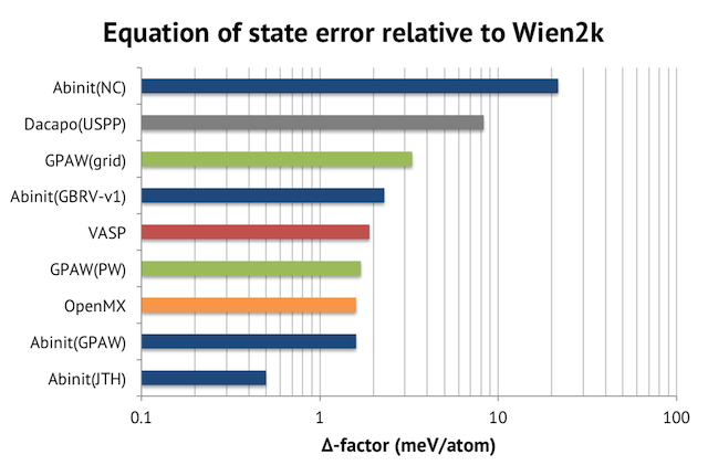
OpenMX is an “order-N” DFT code with numerical pseudo-atomic basis sets and pseudopotentials. It takes a similar approach to solving the DFT problem as the SIESTA, ONETEP, and CONQUEST codes. What directed my attention towards OpenMX was a presentation at the SC13 conference showing excellent parallel scaling on the K computer, and the possibility to get very accurate solutions with the LCAO basis if necessary, as evident in the delta-code benchmark, which I wrote about earlier. It is also available under an open-source GPL license, unlike the other codes.

Installing

OpenMX is now available on Triolith. The code is written in straight C and was easy to compile and install. My changes to the makefile were:

CC = mpiicc -I$(MKLROOT)/include/fftw -O2 -xavx -ip -no-prec-div -openmp 
FC = mpiifort -I$(MKLROOT)/include/fftw -O2 -xavx -ip -no-prec-div -openmp
LIB = -mkl=parallel -lifcoremt

I used the following combination of C compiler, BLAS/LAPACK and MPI modules:

module load intel/14.0.1 mkl/11.1.1.106 impi/4.1.1.036

Initial tests

To get a feel of how easy it would be work with OpenMX, I first tried to set up my trusty 16-atom lithium iron silicate cell and calculate the partial lithium intercalation energy (or the cell voltage). This requires calculating the full cell, Li in bcc structure, and a partially lithiated cell; with spin polarization. To get the cell voltage right, you need a good description of both metallic, semiconducting, and insulating states, and an all-electron treatment of lithium. The electronic structure is a bit pathologic, so you cannot expect to get e.g. SCF convergence without some massaging in most codes. For example, so far, I have been able to successfully run this system with VASP and Abinit, but not with Quantum Espresso. This is not really the kind of calculation where I expect OpenMX to shine (due to known limitations in the LCAO method), but it is a useful benchmark, because it tells you something about how the code will behave in less than ideal conditions.

With the help of the OpenMX manual, I was able to prepare a working input file without too much problems. I found the atomic coordinate format a bit too verbose, e.g. you have to specify the spin up and spin down values for each atom individually, but that is a relatively minor point. As expected, I immediately ran into SCF convergence problems. After playing around with smearing, mixing parameters and algorithms, I settled with the rmm-diisk algorithm with a high Kerker factor, long history, and 1000K electronic temperature. This lead to convergence in about 62 SCF steps. For comparison, with VASP, I got convergence in around 53 SCF steps with ALGO=fastand linear mixing. From the input file:

scf.Mixing.Type rmm-diisk
scf.maxIter 100
scf.Init.Mixing.Weigth 0.01
scf.Min.Mixing.Weight 0.001
scf.Max.Mixing.Weight 0.100
scf.Kerker.factor 10.0
scf.Mixing.StartPulay 15
scf.Mixing.History 30
scf.ElectronicTemperature 1000.0

The choice of basis functions is critical in OpenMX. I recommend the paper by M. Gusso in J. Chem. Phys. for a detailed insight into the quality of the OpenMX basis set vs plane-waves. From quantum chemistry codes, I know that double-zeta basis will get you qualitatively correct results, but triple-zeta basis and above is required for quantitative results. It also seems imperative that you always have at least one d-component. I tried three combinations: s2p1+d (SVP quality), s2p2d1+f (DZP quality), and s3p3d3+f (TZP quality). The resulting cell voltages are shown below. The voltages are expected to decrease as the basis set size increases due overbinding from basis set superposition errors.

s1p1+d:   3.85 V
s1p1+d:   3.40 V (counterpoise correction)
s2p2d1+f: 3.14 V 
s2p2d1+f: 3.00 V (counterpoise correction) 
s3p3d3+f: 2.77 V (counterpoise correction)

For comparison, the converged VASP result with 550 eV and PREC=accurate is 2.80 V, meaning that the s3p3d3-level calculation is quite accurate. This confirms the delta-code benchmark study, where OpenMX calculations were shown to be as accurate as those of VASP, provided that a big basis set is used. In terms of speed, however, the results are not that impressive, on one Triolith compute node with 16 cores, VASP runs this 16-atom cell in 18 seconds at 500eV, whereas OpenMX with s3p3d3 basis takes 700 seconds! We will see, however, in the next section, that the outcome is different for large systems.

512-atom carbon nanotube

I think that carbon nanotubes (and other nanostructures) are a better fit for order-N approaches. For this purpose, I set up a (16,0) nanotube with 512 atoms including terminating hydrogens. It is stated in the OpenMX manual that you need at least 1 atom per MPI process, so ideally we could scale up to 512 cores with MPI, and possibly more with OpenMP multithreading.

Here, I choose DZP level basis set for OpenMX:

<Definition.of.Atomic.Species
C C6.0-s2p2d1  C_PBE13
H H6.0-s2p2d1  H_PBE13
Definition.of.Atomic.Species>

I believe that this is a slightly weaker basis set than what you would get in a standard VASP approach, so for the corresponding VASP calculation, a “rough” basis set of ENCUT=300 and PREC=Normal was chosen. For reference, the ENMAX value in the carbon POTCAR is 400 eV, which is what you would normally use. The calculations are spin-polarized. OpenMX reaches SCF convergence in 46 cycles using a similar scheme as above, and the VASP calculation converges in 34 cycles with the standard ALGO=fast. Both programs agree on a magnetic moment of 9.5-10.0.

In terms of performance, regular order-N(3) DFT in OpenMX is about as fast as in VASP, at least for wider parallel jobs:

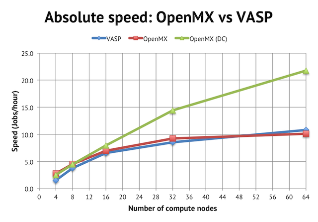
We reach a peak speed of about 10 jobs/hour (or 10 geometry optimization steps per hour) on NSC’s Triolith. Interestingly, for the narrowest job with 4 compute nodes, OpenMX was almost twice as fast as the corresponding VASP calculation, implying that the intra-node performance is very strong for OpenMX, perhaps due to the use of hybrid OpenMP/MPI. Unfortunately, the calculation runs out of memory on less than 4 compute nodes, so I couldn’t test anything smaller (see more below).

The main benefit of using OpenMX is, however, the availability of linear scaling methods. The green line in the graph above shows the speed achieved with the order-N divide-conquer method (activated by scf.EigenvalueSolver DC in the input file). It cuts the time to solution by half, reaching more than 20 jobs/hour, but please note that the speed for narrow jobs is the same as regular DFT, so the main strength of the DC method seems not to be in improving serial (or intra-node performance) but rather in enabling better parallel scaling.

The impact on parallel scalling is more evident if we normalize the performance graph to relative speeds vs the 4-node jobs:

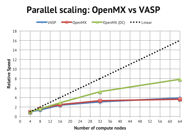
Regular DFT in VASP and OpenMX flattens out after 16 compute nodes, which is equivalent to 256 cores in total or 2 atoms/core, whereas with the linear scaling method, it is possible to beyond that.

Memory consumption

The main issue I had with OpenMX was memory consumption. OpenMX seems to replicate a lot of data in each MPI rank, so it is essential to use the hybrid MPI/OpenMP approach to conserve memory. For example, on 4 compute nodes, the memory usage looks like this for the calculation above:

64 MPI ranks without OpenMP threads = OOM (more than 32 GB/node)
32 MPI ranks with 2x OpenMP threads = 25 GB/node
16 MPI ranks with 4x OpenMP threads = 17 GB/node
 8 MPI ranks with 8x OpenMP threads = 13 GB/node

with 2x OpenMP giving the best speed. For wider jobs, 4x OpenMP was optimal. This was a quite small job with s2p2d1 basis and moderate convergence settings, so I imagine that it might be challenging to run very accurate calculations on Triolith, since there is only 32 GB memory in most compute nodes.

Of course, adding more nodes also helps, but the required amount of memory per node does not strictly decrease in proportion to the number of nodes used:

  4 nodes (2x OpenMP) = 25 GB/node
  8 nodes (2x OpenMP) = 21 GB/node
 16 nodes (2x OpenMP) = 22 GB/node
 32 nodes (2x OpenMP) = 18 GB/node

So when you are setting up an OpenMX calculation, you need to find the right balance between the number of MPI ranks and OpenMP threads in order to get good speed without running out of memory.

Conclusion

In summary, it was a quite pleasant experience to play around with OpenMX. The performance is competitive, and there is adequate documentation, and available example calculations, so it is possible to get started without a “master practitioner” nearby. For actual research problems, good speed and basic functionality is not enough, though, as usually, you need to be able to calculate specific derived properties, and visualize the results in a specific way. I noticed that there are some post-processing utilities available, even inside OpenMX itself, and among the higher level functionality, there is support for relativistic effects, LDA+U, calculation of exchange coupling, electronic transport, NEB and MLWFs, so I think many of the modern needs are, in fact, satisfied.

One common question we get is “Why have my jobs been waiting in the queue for so long?” Upon investigation, it usually transpires that that the user is a member of a project that has run a lot of jobs recently. As a result, the job scheduler will suppress the priority of the newly queued jobs in order to let other projects have a chance of running. We have elaborated a bit on how Triolith’s queue system works on the NSC web page. I specifically recommend reading the section titled “How can I adapt the job scheduling to my workflow?”. The essence of it is:

There is no limit on how much a project can run in a month. But the more you run, the lower your priority will be, so the harder it will be to run the next job.

The relationship is actually non-linear, which is illustrated below:

The queue time in the sketch is a normalized number, but you can imagine it as being days. The percentage representing the project usage is the actual core hours used during the last 30-day period divided by the given allocation, i.e. running 15,000 core hours when having been allocated 10,000 core hours/month by SNAC is 150% usage.

The key insight here is that running more than one’s allocation results in queue times approaching infinity. But note that the allocation, in terms of core hours/month is not a hard limit. It is possible to run more jobs, for example reaching 150% or 200% of your allocated hours for a month. It is even possible to do this consistently over several months if other projects relinquish their core hours. But borrowing from other projects comes at a cost: if your project is always above the allocated usage, the job priority is also always low as a direct result, implying long queue times, as shown in the sketch above.

This means that it is critical for a PI to manage the project to ensure that adequate resources are available when the participants need them. For example, if a PhD student needs to perform a large set of calculations next month in order to finalize their thesis, the PI must prevent the other project members from overusing the project during the current month and accumulating a low priority for everyone as a result. In certain cases, it might even be prudent to underuse the project in order to save up for a priority boost later.

Below, I will show two ways to monitor how the core hours are being used. That will hopefully be helpful in doing capacity planning and manage resource use over time.

The projinfo command

On Triolith (and all other SNIC systems), there is command called projinfo, which reveals the current status of the projects that you are a member of. Here is the output of a hypothetical SNIC project that would suffer from low priority and long queue times:

[x_secun@triolith1 ~]$ projinfo
Project             Used[h]   Current allocation [h/month]
   User
-----------------------------------------------------
snic2014-XX-YY         320807.82              250000
   x_prima               5877.88
   x_secun                  0.34
   x_terti              12229.15
   x_quart              22312.09
   x_quint              23944.71
   x_sextu              75189.68
   x_septi             181253.97

The two most important numbers are the ones in the top, which accounts for the actual usage (320k core hours) over the last 30 days and the target allocation (250k). Note that the first number is an average over a 30-day sliding window, not the number of hours used since the start of the month. Again, it is the relation between the core hours used vs the project’s allocation that controls the priority of jobs. In this case, the priority for all users in the project will be very low. The reason is that the project, as a whole, has overused its allocation. In order to balance the books, this project would need to run less than their allocation during the following month, so that the average value becomes closer to 250k core hours/month. It is the job of the queue system to enforce this through job priorities.

Inspecting project use over time

The projinfo command shows only the most recent 30-day period. For long-term statistics, you can log in to NSC Express. There, it is possible to inspect the historical use of resources for a project per month. The graphs are accessed by clicking on a project name in the table in the “Projects” section of your personal NSC Express page. For example:

Here, one could imagine that around November-December, the queue time situation must have been particularly bad, whereas the other months were more in line with the allocated use and most likely more tolerable.

A new version of VASP, denoted vasp.5.3.5 31Mar14 was released in the beginning of April. Swedish HPC users can find 5.3.5 installed on NSC’s Triolith and Matter clusters, and at PDC’s Lindgren. So what is new? The release notes on the VASP community page mentions a few new functionals (MSx family meta-GGAs, BEEF and Grimme’s D3) together with many minor changes and bug fixes.

The first installation of VASP 5.3.5 binaries at NSC is available in the expected place, so you can do the following in your job scripts:

mpprun /software/apps/vasp/5.3.5-31Mar14/default/vasp

You can also do module load vasp/5.3.5-31Mar14, if you prefer to use modules.

The installation and compilation was straightforward with Intel’s compilers and MKL, but I did not have much success with gcc/gfortran (4.7.2) as usual. Even after applying my previous patches for gfortran, the compiled binary crashed due to numerical errors.

It is also worth mentioning that some recent MPI-libraries now assume MPI version 2.2 standards compliance by default. This is the case with e.g. Intel MPI 4.1, which we use on Triolith. Unfortunately, VASP is not fully compliant with the MPI standard, as there are places in the code where memory buffers overlap, which results in undefined behavior. You can see errors like this when running VASP:

Fatal error in PMPI_Allgatherv: Internal MPI error!, error stack:
...
MPIR_Localcopy(381).......: memcpy arguments alias each other, dst=0xa57e9c0 src=0xa57e9c0 len=49152

Some of the problems can be alleviated by instructing the MPI runtime to assume a different MPI standard. For Intel MPI, one can set

export I_MPI_COMPATIBILITY=4

to force the same behavior as with Intel MPI 4.0. This seems to help with VASP. If we get reports of much problems like this, I will install a new version of VASP 5.3.5 with the old Intel MPI as a stopgap solution.

The Intel-compiled version of 5.3.5 ran through the test suite that I have without problems, implying that the results of 5.3.5 remain unchanged vs 5.3.3 for basic properties, as we expect. The overall performance appears unchanged for regular DFT calculations, but hybrid calculations run slightly faster now. There is also preliminary support for NPAR for Hartree-Fock-type calculations. I played around with it using a 64-atom cell on 64 cores, but setting NPAR actually made it run slower on Triolith, so I suppose k-point parallelization is still much more efficient for hybrid calculations.

How accurate is DFT in theory and in practice? There has been some reviews on the former, comparing calculations of a given DFT program with experiments, but not as much of the latter – comparing the numerical approximations inherent in different DFT codes. I came across a paper taking both of these aspects into account. The paper is titled “Error Estimates for Solid-State Density-Functional Theory Predictions: An Overview by Means of the Ground-State Elemental Crystals”, written by K. Lejaeghere et al. More information about their project to compare DFT codes can be found at their page at the Center for Molecular Modeling at the University of Gent.

Their approach to compare DFT codes is to look at the root mean square error of the equations of state w.r.t. the ones from Wien2K. They called this number the “delta-factor”. The sample set is the ground-state crystal structures of the elements H-Rn in the periodic table. I have plotted the outcome below, which is to be interpreted as the deviation from a full-potential APW+lo calculation, which is considered as the exact solution. Please note the logarithmic scale on the horizontal axis.

My observations are:

• Well-converged PAW calculations with good atomic setups are very accurate. Abinit with the JTH library achieves a delta value of 0.5 meV/atom vs Wien2K. As the authors put it in the paper: “predictions by APW+lo and PAW are for practical purposes identical”.
• Norm-conserving pseudopotentials (NC) with plane-wave basis set are an order of magnitude worse than PAW. The numerical error is of the same magnitude as the intrinsic error vs experiments for the PBE exchange-correlation potential (23.5 meV/atom).
• VASP is no longer the most accurate PAW solution. Similar, or better, quality results can now be arrived at with Abinit and GPAW.
• The quality of the PAW atomic setups matters a lot. Compare the results for Abinit (blue bars in the graph) with different PAW libraries. I think this explains why VASP has remained so popular – only recently did PAW-libraries which surpass VASP’s built-in one become available.
• The PAW setups for GPAW are of comparable quality to VASP’s, but GPAW’s grid approach seems to be detrimental to numerical precision. GPAW with plane-wave (PW) basis gets 1.7 meV/atom vs 3.3 meV/atom using finite differences.
• OpenMX (pseudo-atomic orbitals + norm-conserving PPs) performs surprisingly well, matching the PAW results. I noticed that the calculations employed very large basis sets, though, which should slow down the speed significantly.

Another relevant aspect is the relative speed of the different codes. Do you have to trade speed for precision? The paper does not mention the accumulated runtime for the different data sets, which would otherwise have made an interesting “price/performance” analysis possible.

Before, I tried to compare the absolute performance and the parallel caling of Abinit and VASP, reaching the conclusion that Abinit was significant slower. Perhaps the improved precision is the reason why? Regarding GPAW, I know, from unpublished results, that GPAW exhibits similar parallel scaling to VASP and matches the per core performance, but SCF convergence can be an issue. OpenMX can be extremely fast compared to plane-wave codes, but the final outcome critically depends on the choice of the basis set.

I am putting GPAW and OpenMX on my list of codes to benchmark this year.

On Triolith, we have the Perf profiler tool installed on all computer nodes. It is pretty neat, because it allows you to look into your running jobs and see what they are doing, without recompiling or doing a special profiling run. This can be quite useful for locating bottlenecks in the code and to quickly check whether jobs appears to be running efficiently.

Here is a rundown on how do it. Suppose we are running a job on Triolith. First, we need to find out on which nodes the job is running on. This information is availble in the squeue output in the “NODELIST” column.

[pla@triolith1 ~]$ squeue -u pla
 JOBID PARTITION     NAME     USER  ST       TIME  NODES NODELIST(REASON)
 1712173  triolith _interac      pla   R       0:17      2 n[2-3]

If you are running a job on a node, you are allowed to use ssh to log in there and check what is going on. Do that!

[pla@triolith1 ~]$ ssh n2
....(login message)...
[pla@n2 ~]$ 

Now, running the top command on the node, will show us that they we are busy running VASP here, as expected.

The next step is to run perf top instead. It will show us a similar “top view”, but of the subroutines running inside all of the processes running on the node. Once you have started perf top, you will have to wait at least a few seconds to allow the monitor to collect some samples before you get something representative.

If your program is compiled to preserve subroutine names, you will see a continuously updating list of the “hot” subroutines in your program (like above) even including calls to external libraries such as MKL and MPI. The leftmost percentage number is the approximate amount of time that VASP, in this case, is spending in that particular subroutine. This specific profile looks ok, and is what I would expect for a properly sized VASP run. The program is spending most of the time inside libmkl_avx.so doing BLAS, LAPACK, and FFTWs operations, and we see some a moderate amount of time (about 10% in total) in libmpi.so doing and waiting for network communications.

For something more pathological, we can look at a Quantum Espresso phonon calculation, which I am deliberately running on too many cores.

Here, something is wrong, because almost 70% of the time seems to be spent inside the MPI communications library. There is actually very little computation being done – these compute nodes are just passing data back and forth. This is usually an indication that the job is not parallelizing well, and that you should run it on less nodes, or at least use less cores per node. In fact, here I was running a phonon job of a simple metal on 32 cores on 2 compute nodes. The runtime was 1m29s, but it would have run just as fast (1m27s) on a single compute node with just 4 cores. The serial runtime, for comparison, was 4m20s. Now, 1 minute on 1 compute is not much time saved, but imagine the effect if this was a job running on 16 compute nodes for one week. That is a saving of 20,000 core hours.

There are much more things you can do with perf, for example, gathering statistics from processor performance counters using perf stat, but for starters, I would suggest using it as a routine check when preparing new jobs to run on the cluster. For big jobs using hundreds of thousands of cores, I would always recommend doing a real parallel scaling study, but for small jobs, it might not be worth it. That is when perf top comes in handy.