When I attended the supercomputing conference last year, I talked to many people in the booths and discovered that despite all the talk about petascale and exascale computing, VASP calculations are still a big part of what most supercomputing sites in the world are serving to their users. This seems to apply everywhere, not only in Sweden. But surprisingly, some described VASP as being “hugely problematic”, claiming that the parallel scalability was extremely bad – 64 cores maximum under any circumstances. In my experience, though, there is no problem running VASP on thousands of CPU cores, provided that you have a sufficiently large cell. My rule of thumb is that you need at least one atom per core, so if you have a supercell with a few thousand atoms, you can in fact run it with acceptable speed on current clusters by running it in a massive parallel fashion. It is true that a typical electronic structure calculation is not going to be that big, but I believe there are certain use cases for cells that big, for example when studying very low dopant concentrations, or simulations of nanostructures.

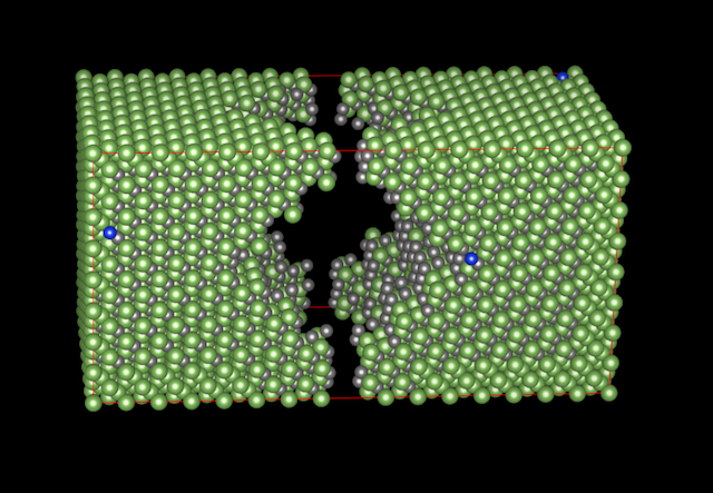
To show what would be possible for our users, provided they had a sufficiently large allocation of core hours, I decided to test the limits by setting up a new benchmark calculation: a 5900-atom supercell of Si-doped GaAs. It has dopants in random positions, and a big void in the middle, so there is no symmetry in this structure. In total, there is 5898 atoms, 23564 electrons, and about 14700 bands (depending on the number of cores employed).

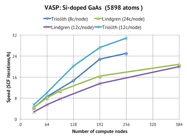
The questions at issue are: would you be able to run this cell with VASP given a big enough allocation on a Sweden HPC resource like Triolith or Lindgren; and from technical point of view, can you even run VASP on that many cores in the first place? The answer is “yes” to both questions, as is evident from the graph below. Employing 256 nodes and 3072 cores of Triolith gives us a speed of roughly 30 SCF iterations per hour, and with Lindgren, the number is 20 SCF steps/hour using 384 nodes and 9216 cores (i.e. 25% of the full machine).

I would like to emphasize that no special magic is required to get a parallel scaling like that. It is the standard VASP source code compiled with the Intel toolchain, as described in the guides I have published. There were no special runtime settings other than NPAR=number of nodes and switching to RMM-DIIS exclusively (IALGO=48).

To illuminate in more detail, what is going on below the surface, we can look at the time profile of different subroutines. A regular VASP calculation will spend most of its time doing electronic minimization (subroutine RMM-DIIS or equivalent), but that is not what we find here. A breakdown from the 384-node run on Lindgren shows:

ORTCH (orthogonalization of wavefunctions) 40%
EDIAG (subspace diagonalization)           50%
RMM-DIIS (electronic minimization)         10%

Most of the time is spent orthogonalizing and deconstructing linear combinations of Kohn-Sham orbitals! At first, I suspected that this was a parallel scaling issue with SCALAPACK, similar to what I found for smaller systems, but the time profile is almost the same on 32 nodes, so evidently, those are real, new bottlenecks that come into play. The reason is, I believe, that ORTCH and EDIAG formally scales as N^3, and that finally, they seem to have overtaken the other terms scaling as N² and N² log N. During the DFT world record (?) featuring 107292 atoms on the K computer, Hasegawa et al observed the same effect, with the conjugate-gradient minimizing part only being 1% of the computational cost.

To me, this proves that the computationally intensive parts of VASP are very well parallelized and that there are no serial parts that overtake the computations as the calculation is scaled up. The trick is rather that you need to scale up your systems as well, should you want to run big.

A new version (v4) of my test suite for VASP is now available. You can find it on GitHub:

https://github.com/egplar/vasptest

This time, I decided to rewrite it from scratch, and drop the beetest testing framework in favor of using Python Behave instead. The extra work involved in maintaining my own testing software was not worth it when it was possible to get the same, or better, flexibility with an existing solution.

With behave, the tests are now written in plain English, which is much easier to read compared to the earlier XML format. The actual test code now looks like this:

...
Scenario: Fe-bcc
When I run VASP with a maximum of 8 ranks
Then the total energy should be -8.231456 +/- 1.0e-5 eV
and self consistency should be reached in 16 iterations
and the Fermi energy should be 9.629837 +/- 0.01 eV
and the pressure should be -39.29 +/- 0.1 kB
and the xx component of the stress tensor should be -39.28618 +/- 0.1 kB
and the yy component of the stress tensor should be -39.28618 +/- 0.1 kB
and the zz component of the stress tensor should be -39.28618 +/- 0.1 kB
and the xy component of the stress tensor should be 0.0 +/- 0.01 kB
and the magnetic moment should be 2.2095 +/- 0.01 uB
and the point group symmetry should be O_h
and the XML output should be valid
...

When the tests are run, the text above is translated into Python code which does the actual inspection and checking of the output files. Hopefully, this change will make it easier for other people to make changes and write their own test cases.

In addition to the code rewrite, there are several new test cases in version 4. They are aimed at testing the GW, hybrid-DFT, and density of states functionality. There is more information on the vasptest page.

I promised a third round of Quantum Espresso (QE) benchmarking vs VASP, where I would try out some large supercells. Supposedly, this is where QE was supposed to shine, judging from the reported benchmarks on their home page. They show a 1500-atom system consisting of a carbon nanotube with 8 porphyrin groups attached. It shows good scaling up to 4096 cores on a Cray XT4 system.

My endeavor did not produce beautiful scaling graphs, though, as I tried several big supercells in QE with the PAW method, but were unable to get them to run reliably. They either run out of memory, or crash due to numerical instabilities. In the end, I decided to just pick the same 1532-atom carbon nanotube benchmark displayed above. It is a calculation with ultrasoft pseudopotentials, which would be unfair to compare with a VASP calculation with PAW. But since there is a special mode in VASP to emulate ultrasoft potentials, activated by LMAXPAW=-1, we can use that one make to the comparison more relevant.

In terms of numerical settings, we have 5232 electrons and the plane wave cutoff encutwfc in the QE reference calculation is 25 Ry (340 eV), with encutrho 200 Ry. The memory requirements are steep and VASP runs out of of memory on 8 nodes, but manages to run the simulation on 16 nodes, so the total memory requirement is between 256GB and 512GB. QE, on the other hand, cannot run the simulation even on 50 nodes, and it is not until I reduce encutwfc to 20 Ry and run with 50 nodes using 8 cores/node that I am able to fit in on Triolith with 32GB/node. This means that the memory requirements are significantly higher for QE than VASP. The “per-process dynamical memory” is reported as ca 1.1 GB in the output files, but in reality, it is using closer to 3 GB per process on 50 nodes.

Now, to performance results. The good news is that this system scales beautifully with VASP, but the bad news is that it does not look that great with QE. With VASP, I used no other tricks than the tried and tested NPAR=nodes, and for QE, I tested -ntg=[1-4] and used similar SCALAPACK setups (-ndiag 100 and -ndiag 196) as in the reference runs. -ntg=1 turned out to be optimal here, as expected (400-800 cores vs 500ish grid points in the z direction).

When looking at the scaling graph, we have near linear scaling in a good part of the range for VASP. It is quite remarkable that you can get ca 10 geometry optimization steps per hour on such a large system using just 4% of Triolith. This means that doing ab initio molecular dynamics on this system would be possible on Triolith, provided that you had a sufficiently large project allocation (several million core hours per month).

The high memory demands and instability of QE prevented me from doing a proper scaling study, but we have two reference points at 50 and 100 compute nodes. There is no speedup from 50 to 100 nodes. This is unlike the study on the old Cray XT4 machine, where the improvement was in the order of 1.5x going from 1024 to 2048 cores. So I am not really able to reproduce these results on modern hardware. I suspect that what we are seeing is an effect of faster processors. In general, the slower the compute node is, the better the scaling will be, because there is more work to be done relative to the communication. An alternative theory is that I am missing something fundamental in running PWscf in parallel, despite having perused the manual. Any suggestions from readers are welcome!

In conclusion, the absolute speed of Quantum Espresso using 50 compute nodes with a large simulation cell is less than half of that of VASP, which further confirms that it does not look attractive to run large supercells with QE. You are also going to need much more memory per core, which is a limitation on many big clusters today.

Update 2013-12-19: A reader asked about the effective size of the fast Fourier grids used, which is what actually matters, rather than the specified cut-of (at least for VASP). In the first results I presented, VASP actually used a 320x320x320 FFT grid vs the 375x375x375 in QE. To make the comparison more fair, I reran the data points for 50 and 100 nodes with PREC=Accurate in VASP, giving a 432x432x432 grid, which is what you are currently seeing in the graph above. The conclusion is still the same, though.

To further elaborate, I think that one of the main reasons for the difference in absolute speed (but not parallel scalability) is the lack of RMM-DIIS for matrix diagonalization in QE. In the VASP calculations, I used IALGO=48, which is RMM-DIIS only, but for QE I had to use Davidson iterative diagonalization. In the context of VASP, I have seen that RMM-DIIS can be 2x faster than Davidson for wide parallel runs, so something similar could apply for QE as well.

Next week, I am off to Denver, Colorado to participate in The Supercomputing Conference (SC13). I will also attend HP-CAST and the Intel HPC Roundtable. I am always interested in meeting other people working with ab initio/electronic structure software. Send me an email if you want to meet up.

Here comes a more generic recipe for installing and compiling VASP using only open-source tools (i.e. without Intel’s Fortran compiler and MKL). This chould be useful if you want to run smaller calculations on a laptop or an office machine. Below follows how I did it on Ubuntu 13.10 with GCC/Gfortran, OpenMPI, OpenBLAS, FFTW and Netlib SCALAPACK. Please note that compiling VASP with gfortran is not recommended or supported by the VASP developers. From what I can tell, it appears to work, but I have only done limited testing.

Prerequisites

First of all you need the VASP source code, which you get from the VASP home page:

http://www.vasp.at/ 

Then we need to install some Ubuntu packages. Install either through the Synaptic program or apt-get in the terminal.

• build-essential
• gfortran
• openmpi1.6-bin
• libopenmpi1.6-dev
• libfftw-double3
• libfttw-single3
• libfftw-dev

This is starting from a completely new Ubuntu installation. If you have done any programming on your machine before, some of these packages could already be installed. For other Linux distributions, you will need to find out the names of the corresponding packages. They should be similar, except for “build-essential”, which is specific to Debian.

I did not have much success using Ubuntu’s BLAS/LAPACK/ATLAS, so we will need to download the latest OpenBLAS and compile it ourselves from source. The same applies to SCALAPACK, which we have to tie together with our OpenBLAS and the system OpenMPI installation.

OpenBLAS

Download the latest OpenBLAS tarball from

http://www.openblas.net/

After decompressing it, you will have a directory called “xianyi-OpenBLAS-….”. Go inside and check the TargetList.txt file. You will have to decide which processor architecture target is appropiate for your processor. For a new Intel processor, “SANDYBRIDGE” should be best, and for a new AMD processor, “BULLDOZER”. Here, I choose the safe and conservative option “CORE2”, which should work on any recent processor. Then we compile with make.

make FC=gfortran CC=gcc USE_THREAD=0 TARGET=CORE2

This should produce a library called libopenblas_core2-r0.2.8.a (or similar). Make note of the directory in which you compiled OpenBLAS, you will need it later. Mine was “/home/pla/build/xianyi-OpenBLAS-9c51cdf”

SCALAPACK

Download the latest SCALAPACK tarball from Netlib.org. To compile it, we need to set up a SLmake.inc file containing some configuration parameters. Start by copying the SLmake.inc.example file. You need to update the BLASLIB and LAPACKLIB variables and insert a direct reference to your OpenBLAS compilation.

CDEFS         = -DAdd_
FC            = mpif90
CC            = mpicc 
NOOPT         = -O0
FCFLAGS       = -O3
CCFLAGS       = -O3
FCLOADER      = $(FC)
CCLOADER      = $(CC)
FCLOADFLAGS   = $(FCFLAGS)
CCLOADFLAGS   = $(CCFLAGS)
ARCH          = ar
ARCHFLAGS     = cr
RANLIB        = ranlib
SCALAPACKLIB  = libscalapack.a
BLASLIB       = -L/home/pla/build/xianyi-OpenBLAS-9c51cdf -lopenblas
LAPACKLIB     = $(BLASLIB)
LIBS          = $(LAPACKLIB) $(BLASLIB)

This should be enough to get SCALAPACK to compile by typing “make”. In the end, you should get a libscalapack.a file.

Compiling VASP

Proceed to compile VASP with gfortran according to the previous guide. You need to apply the source code patches described there, otherwise it is straightforward. If you have never compiled VASP before, looking through one of the more detailed system specific guides in the VASP compile section might help.

The makefiles and the source code patch I used are available for download: vasp-ubuntu.tar.gz.

Some highlights (update the paths if necessary):

FFLAGS = -ffree-form -ffree-line-length-0  -fno-second-underscore -I/usr/include

We need to include -I/usr/include to pick up the FFTW header file.

BLAS= ../../xianyi-OpenBLAS-9c51cdf/libopenblas-core2.a

And refer to the BLAS/LAPACK library from our OpenBLAS installation.

CPP    = $(CPP_) -DMPI  -DHOST=\"LinuxGfort\" \
     -DCACHE_SIZE=4000 -Davoidalloc -DNGZhalf \
     -DMPI_BLOCK=262144 -Duse_collective -DscaLAPACK -DMINLOOP=1  

And set the precompiler flags. In the MPI section of the makefile, there should be a reference to our compiled SCALAPACK:

SCA=/home/pla/build/scalapack-2.0.2/libscalapack.a

Running VASP

The binaries you compile are MPI-enabled, so they should be launched with mpirun. For example:

mpirun -np 4 ~/build/vasp-5.3.3/vasp.5.3/vasp

You will probably find that the --bind-to-core option will help performance.

mpirun -np 4 --bind-to-core ~/build/vasp-5.3.3/vasp.5.3/vasp

If you have dual socket workstation, similar to a compute cluster node, I recommend trying:

mpirun -np 16 --bind-to-core --npersocket 8 ~/build/vasp-5.3.3/vasp.5.3/vasp

When doing standard double precision floating point operations in C or Fortran, you can expect 15-17 significant digits. But what do you do when 15 decimals are not enough? The GNU multiple precision arithmetic library is go-to library when you need not 15, but thousands of decimals, but for more modest needs, quadruple precision (128 bits), might be enough. In Fortran, 128 bits is REAL*16, and in C we can access it by the type __float128. These may not be availabe in all compilers, but GCC (4.6 and newer) and Intel C/Fortran do support it. According to the GCC manual, we can expect it to be “an order of magnitude or two slower” than double precision.

I decided to test the quad precision by doing a simple matrix-matrix multiplication test. Two 256x256 matrices are initialized with trigonometric expressions and then multiplied by each other. It is straightforward to change the program into quad precision: the doublearrays should be declared as __float128, the trig. functions are called cosq/sinq, and we need to use the special function quadmath_snprintf to print the numbers to the screen. (In Fortran, you don’t even need to use a different print function.)

For simplicity, I look specifically at the decimal expansion of one matrix element (0,0). With gcc, I get

$ gcc -o matmul_double -O3 -mavx -std=c99 matmul_double.c -lm
$ ./matmul_double
Matrix size: 256 by 256 (double precision).
Time: 0.010 seconds (3355.4 MFLOP/s)
C(0,0)-diagnostic: -0.0939652685936642

gcc -o matmul_quad -std=c99 -O3 -mavx matmul_quad.c -lquadmath -lm
./matmul_quad
Matrix size: 256 by 256 (quad precision).
Time: 4.140 seconds (8.1 MFLOP/s)
C(0,0)-diagnostic: -0.093965268593662358578620940776

which confirms that __float128 works in gcc, but with significant speed penalty. In this case, the difference in runtime is around 1000x.

Does Intel’s C compiler fare better?

$ icc -o matmul_double -std=c99 -O3 -xavx mmul_double.c -lm
$ ./matmul_double
Matrix size: 256 by 256 (double precision).
0.000 seconds (inf MFLOP/s)
C(0,0)-diagnostic: -0.0939652685936624

$ icc -o matmul_quad -std=c99 -O3 -mavx -I/software/apps/gcc/4.7.2/lib/gcc/x86_64-unknown-linux-gnu/4.7.2/include -L/software/apps/gcc/4.7.2/lib64/ matmul_quad.c -lquadmath -lm
$ ./matmul_quad
Matrix size: 256 by 256 (quad precision).
0.880 seconds (38.1 MFLOP/s)
C(0,0)-diagnostic: -0.093965268593662358578620940776

Yes, it is evident that the quad precision floating maths runs a few times faster with ICC, even though the same underlying library is used.

If we actually look at the decimals, and compare the results, we find something interesting. The quad precision results from GCC and ICC are identical, which is assuring, but the double precision binary compiled by ICC delivers higher precision, despite using very high optimization.

GCC(double) -0.09396526859366|42
ICC(double) -0.09396526859366|24
GCC(quad.)  -0.09396526859366|2358578620940776
ICC(quad.)  -0.09396526859366|2358578620940776

Lowering GCC’s optimization did not help, and gcc is not supposed to introduce any unsafe mathematical operations unless explicitly enabled by -ffast-math or -Ofast in the first place, so it is unclear to me where the difference comes from. Typically, fluctuations in the last decimal is not a problem in practice for many codes. There are many that run fine with e.g. gcc’s -ffast-math, but if you are struggling with ill-conditioned matrices, every decimal could count.

Are bigger servers better for high-performance computing? It is often assumed that communication between processors within a compute node must be faster than using Infiniband networking in a cluster. Consequently, I come across scientists asking for big shared memory servers, believing that their simulations would run much faster there. In reality, it is not always so. In the previous post, I wrote about how the VASP application is bottlenecked by memory bandwidth. In such cases, compute work and communication will compete with each other for precious resources, with severe performance degradation as a result.

Consider this experiment. Let us first run a VASP compute job with 512 bands on a single compute node using 1 to 16 cores. This will give us a scaling graph showing what kind of improvement you can get by using more cores in a server. Now, for comparison, we run the same job but with only one core per compute node. This means that the 16-core job uses 16 compute nodes and only communicates over Infiniband. Which scenario will be faster?

It turns out that communicating only over Infiniband is superior to shared memory. With 16 cores it gives twice as fast calculations. The reason is simply that we throw more hardware at the problem: our processors can now use all the memory bandwidth for computations, while exchanging data over the Infiniband network instead.

The graph above shows that there is no inherent benefit to run an MPI parallelized application such as VASP on a big server vs smaller servers in a cluster connected by Infiniband. The only advantage you get is the increased total amount of available memory per server.

As a user, you can apply techniques like this to speed up your calculations. For example, by using twice as many nodes, but with half the number of cores on each node. On Triolith, you can do like this:

#SBATCH -N 16
#SBATCH --ntasks-per-node 8

mpprun /software/apps/vasp/5.3.3-18Dec12/default/vasp

This will run your application with 8 cores per compute node, for a total of 128 cores. The improvement in speed compared to using 8 full nodes can be as much as 50%, and you will also have twice as much memory available per processor. The drawback is, of course, that you spend twice the core hours on your calculation. But if it is important to get the results quickly, it might be worth it.

I was recently asked what kind of hardware you should for running VASP calculations. I recommend looking at the configuration of the Triolith cluster at NSC. It was designed to run VASP as big part of the workload, and we did extensive benchmarking to optimize price/performance. An alternative is too look through the supercomputing Top500 list for the most recent entries, to get a feel for what the supercomputing centers are buying at the moment. At Top500, they also have a statistics section where you can follow trends in hardware over time. It is obvious, for example, that big shared memory systems have fallen out of favor.

I recommend is dual-socket servers with low clock frequency Intel Xeon E5 processors, connected by Infiniband networking. Why?

• Type of CPU: At the moment, Intel’s server processors are significantly ahead of AMD’s in terms of performance and energy efficiency. VASP is also very reliant on Intel’s Fortran compiler. This makes Intel processors an optimal choice. It is possible to run VASP on POWER and SPARC processors, but these server platforms are generally not cost efficient for high-performance computing.

• CPU model: VASP is very dependent on high memory bandwidth. It is one of the most memory intensive applications in high-performance computing. This means that you do not need processors with high clock frequency, because they will spend most of their time waiting for data to arrive from memory anyhow. What you need is the cheapest processor model that still comes with maximum memory bandwidth. In the current Xeon E5-2600 series, that is likely to be the 2650 and 2660 models. The quad-core 2643 model could also be interesting, because you typically gain only 25% when going from 8 to 16 cores per node.

• Memory: It is crucial to have 1600 Mhz DDR3 memory, which is currently the fastest memory (1866 Mhz will soon come). All four memory channels should be occupied. Try to get dual rank memory modules if you have only 1 DIMM per memory channel – it will improve performance by ca 5%. Typically, 32 GB of memory is enough (2 GB/core), the reason being that you can easily get an equivalent of 4 GB per core by running with half the number of MPI ranks per node without losing too much performance. But if the majority of jobs are of hybrid type or GW, I would go for 64 GB per server instead.

• Network: A fast network, like Infiniband, is necessary to run VASP in parallel on more than a few nodes. It is difficult to do comparative studies of different network setups due to the amount of hardware required, but in general VASP scales almost perfectly up to 16 compute nodes using both Mellanox and Qlogic (now Intel) Infiniband, so there is no given winner. FDR Infiniband does not significantly improve performance over QDR for VASP in the few tests I was able to do (+16% on a 16 node job spanning two switches), so I would look at it mostly from a price/performance perspective.

Occasionally, I get enquiries about various kinds of scripts for pre- and post-processing of VASP calculations. A comprehensive set of scripts covering the most common tasks is available within the Aflow high-throughput framework for VASP, developed by the Curtarolo group at Duke University.

To use Aflow on Triolith, just load the “vasptools/0.2” module; it will put the aconvasp binary and other scripts such as “vasp2cif” and “vaspcheck” into your PATH.

module load vasptools/0.2

Here are some examples of what can you do with Aflow:

• aconvasp --cart: convert POSCAR from direct to Cartesian coordinates
• aconvasp --data: show basic structure data such as volume, alpha, beta gamma, etc.
• aconvasp --volume 170.0: Change the volume of the cell to 170 A³ .
• aconvasp --clat 5.0 5.0 7.0 90.0 90.0 120.0: convert (a,b,c,alpha,beta,gamma) to Cartesian basis vectors which can be copy-pasted into POSCAR.
• aconvasp --chgdiff CHGCAR.1 CHGCAR.2: subtract charge densities in CHGCAR files. (But it seems to be broken when I test it.)
• aconvasp --supercell 2 2 2: make supercell out of an existing POSCAR.
• aconvasp --swap 0 1: swap coordinates of atomic species 0 and 1 in the POSCAR file.
• aconvasp --spacegroup: spacegroup and symmetry detection.
• aconvasp --cif: generate a CIF file from POSCAR.
• aconvasp --xyz: generate an xyz file from POSCAR.

You can find more information in the full documentation. If you use aconvasp or aflow, don’t forget to cite their paper:

S. Curtarolo, W. Setyawan, G. L. W. Hart, M. Jahnatek, R. V. Chepulskii, R. H. Taylor, S. Wang, J. Xue, K. Yang, O. Levy, M. Mehl, H. T. Stokes, D. O. Demchenko, and D. Morgan, AFLOW: an automatic framework for high-throughput materials discovery, Comp. Mat. Sci. 58, 218-226 (2012).

This week we are running a course in parallel programming with OpenMP at NSC. Joachim Hein from LUNARC is teaching and a few of us from NSC are helping out with the programming labs.

It is often said that parallel programming can be incredibly hard, and that there is currently no reliable way to automatically parallelize an existing serial program. This statement is still true in general, but sometimes, parallel programming can also be embarrassingly easy. Why? Because while automatic parallelization is not perfect, it can still give you some improvement. There are also many subroutines in BLAS, LAPACK and FFTW that are already parallelized, and since many programs rely on these libraries, they can see speed-up on multicore processors by just linking the right library version and setting OMP_NUM_THREADS=X in the shell.

Let us consider the Elk FP-LAPW code . It is written in Fortran90, and has already been parallelized using both OpenMP and MPI. But what could we have done in the hypothetical case of starting out with the serial version of Elk? How good is automatic parallelization? It will surely not get us all the way, but every percent counts, because you essentially get it for free. It is merely a question of finding the relevant compiler flags.

To establish a baseline, I have Elk compiled without any special compiler flags or machine-optimized numerical libraries. This may seem naive and unrealistic, but in reality, it is not uncommon to come across scientific software built without any compiler optimizations flags or optimized linear algebra libraries such as GotoBLAS, MKL, or ATLAS. (In my experience, it is not so much a result of ignorance, but rather technical problems with compilation and/or lack of time for tinkering.)

The test case I am using is the YBCO example distributed with Elk (13 atoms) with the rgkmax parameter increased to 7.0 to get longer runtime.

The first step in our hypothetical example is to simply add “-O3” optimization. This gives us 9% speed boost. The next crucial step is to replace the bundled BLAS, LAPACK and FFT libraries with Intel’s MKL libraries, which improves the speed by 27%. And finally, we activate the compiler’s automatic threaded parallelization, which gives us +80%. The results can then be compared with the production version of Elk for Triolith, which uses aggressive compiler optimizations, MKL libraries, and has manual OpenMP parallelization.

We can see that automatic parallelization gives a modest speed-up of 1.7x using 16 cores on a Triolith compute node. Still, this is not too bad compared with the OpenMP parallelized version which gets 5.0x over the serial version in total, but only 2x of that is actually due to the OpenMP constructs in the code. So essentially, we get half of the parallelization done automatically for free, without having to change any Fortran code.

Another way of looking at this graph is that it can really pay off to spend some time looking into the best way to compile and link a program. The optimized auto-parallel version is 2.5x faster than the naive version built just from the Elk source with integrated numerical libraries.

Most of tricks I used to compile Elk in this example are listed in the Triolith User Guide. If you encounter problems compiling your own program on Triolith, or need help with choosing the best libraries, please don’t hesitate to contact support@nsc.liu.se.