

During the Christmas holidays, I had the oppurtunity to run some VASP benchmarks on Beskow, the Cray XC40 supercomputer currently being installed at PDC in Stockholm. The aim was to develop guidelines for VASP users with time allocations there. Beskow is a significant addition in terms of aggregated core hours available to Swedish researchers, so many of heavy users of supercomputing in Sweden, like the electronic structure community, were granted time there.
For this benchmarking round, I developed a new set of tests to gather data on the relationship between simulation cell size and the appropriate number of cores. There has been concerns that almost no ordinary VASP jobs would be meaningful to run on the Cray machine, because they would be too small to fit into the minimal allocation of 1024 cores (or 32 compute nodes, in my interpretation). Fortunately, my initial results show that this is not case, especially if you use k-point parallelization.
The tests consisted of GaAs supercells of varying sizes, doped with a single Bi atom. The cells and many of the settings are picked from a research paper, to make it more realistic. The supercell sizes were successive doublings of 64, 128, 256, and finally 512 atoms, with a decreasing number of k-points in the Monkhorst-Pack grids (36, 12, 9, 4). I think it is a quite realistic example of a supercell convergence study.
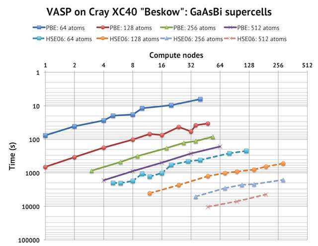
First, please note the scales on the axes. The y-axis is reversed time in logarithmic scale, so upwards represents faster speed. Similarly, the x-axis is the number of compute nodes (with 32 cores each) in log-2 scale. A 256-node calculation is potentially 8192 cores! But in this case, I used 24 cores/node, except for the biggest HSE06 cells, where I had to reduce the number cores per node to gain more memory per MPI rank. The solid lines are PBE calculations and the dashed lines HSE06 calculations. Note the very consistent picture of parallel displacement of the scaling curves: bigger cells take longer time to run and scale to a larger number of compute nodes (although the increase is surprisingly small). The deviations from the straight lines comes from outlier cases where I had to use a sub-optimal value of KPAR, for example, with 128 atoms, 32 nodes, and 12 k-points, I had to use KPAR=4 instead of KPAR=12 to balance the number of k-points. For real production calculations, you could easily avoid such combinations.
The influential settings in the INCAR file were:
NCORE = cores/node (typically 24)
KPAR = MIN(number of nodes,number of k-points)
NSIM = 2
NBANDS = 192, 384, 768, 1536 (which are all divisible by 24)
LREAL = Auto
LCHARG = .FALSE.
LWAVE = .FALSE.
ALGO = Fast (Damped for HSE06)
There were no other special tricks involved, such as setting MPI environment variables or custom MPI rank placement. It is just standard VASP calculations with minimal input files and careful settings of the key parameters. I actually have more data points for even bigger runs, but I have chosen to cut off the curves where the parallel efficiency fell too much, usually to less than 50%. In my opinion, it is difficult to motivate a lower efficiency target than that. So what you see is the realistic range of compute nodes you should employ to simulate a cell of a given size.
If we apply the limit of 32 nodes, we see that a 64-atom GGA calculation might be a borderline case, which is simply to small to run on Beskow, but 128 atoms and more scale well up to 32 compute nodes, which is half a chassis on the Cray XC40. If you use hybrid DFT, such as HSE06, you should be able to run on 64 nodes (1 chassis) without problem, perhaps even up to 4 chassis with big supercells. In that case, though, you will run into problems with memory, because it seems that the memory use of an HSE06 calculation increase linearly by the number of cores I use. I don’t know if it is a bug, or if the algorithm is actually designed that way, but it is worth keeping in mind when using hybrid functionals in VASP. Sometimes, the solution to an out of memory problem is to decrease the number of nodes.
In addition to parallel scaling, we are also interested in the actual runtime. In some ways, it is impressive. Smaller GGA calculations can complete 1 SCF cycle in less than 1 minute, and even relatively large hybrid-DFT jobs can generally be tuned to complete 1 SCF cycle in per hour. In other ways it is less impressive. While we can employ more compute nodes to speed up bigger cells, in general, we cannot always make a bigger system run as fast as a smaller by just adding more compute nodes. For example, an HSE06 calculation will take about two orders of magnitude longer time to run than a GGA calculation, but unfortunately, it cannot also make use of two orders of magnitude more compute nodes efficiently. Therefore, large hybrid calculations will remain a challenge to run until the parallelization in VASP is improved, especially with regards to memory consumption.