

In a previous post, Running big on Lindgren, we saw how VASP could be run with up to 2000 cores if a sufficiently big supercell was used. But where does this limit come from?
What happens is that the fraction of time that a program spends waiting for network communication grows as you increase the number of MPI ranks. When there are too many ranks, there is no gain anymore, and adding more cores only creates communication overhead. This is where our calculation “stops scaling” in everyday speak. In many cases, performance might even go down when you add more cores.
We can see this effect by measuring the amount of time spent in MPI calls. One tool that can do this is the mpiP library. MPIP is simple library that you need to link to your program. It will then intercept any MPI calls from your program and collect statistics. When increasing the number of ranks in a VASP calculation, it can look like this:
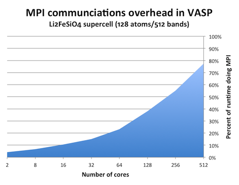
(The graph above was generated from runtimes on the Matter cluster at NSC, but the picture should be the same on Lindgren.) It is clear that this problem cannot be subdivided to arbitrary degree. With 256 and more cores, the individual chunk of work that each core has to do is so small that it takes longer time send to results to other cores than to actually calculate them.
Another way to look at it is to pinpoint where in the program the bad scaling arises. It is often a performance critical serial routine, or an MPI parallelized subroutine, which is heavily dependent on network performance. Conveniently, VASP has built-in timing libraries that measures contributions of several important subroutines in the program. As far as I know, the timings are accurate.
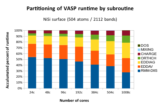
This graph shows the share of the total CPU time spent in each subroutine. “24c” means 24 cpu cores, or one computer node in Lindgren. The maximum number of 1008 cores is equal to 42 compute nodes.
To understand this data, first note that each column is normalized to 100% runtime, because we are not interested in the runtime per se, but rather what happens to individual parts when we run a wide parallel job. Ideally, all the bars should be level. This is because if there is no (or constant) communication overhead, a certain subroutine will always requires the same amount of aggregated compute time, because the actual compute work (without communication) is the same regardless of how many cores we are running on. Instead, we see that some subroutines (EDDIAG/ORTHCH) increase their share of time as we run on more tanks. These are the ones that exhibit poor parallel scaling.
What does EDDIAG and ORTHCH do? They are involved in the so-called “sub-space” diagonalization step. ORTHCH does the LU decomposition and EDDIAG diagonalizes the Hamiltonian in a space spanned by the trial Kohn-Sham orbitals. This procedure is necessary because the RMM-DIIS algorithm in VASP does not give the exact orbitals, but rather a linear combination of the eigenfunctions with the lowest energy. The problem is that this procedure is usually trivial and fast for a small system (the matrix size is NBANDS x NBANDS), but it becomes a bottleneck for large cells.
There is, however, a way parallelize this operation with SCALAPACK, which VASP also employs, but it is well-known that the scalability of SCALAPACK in this sense is limited. It is also mentioned in the VASP manual in several places (link). We can see this effect in the graph, where the yellow fraction stays relatively flat up to 192 cores, but then starts to eat up computational time. So, for now, the key to running VASP in parallel on > 1000 cores is to have many bands. A more long-term solution would be to find an alternative to using SCALAPACK for the sub-space diagonalization.