When Triolith had a service stop recently, I took to the opportunity to explore the Abisko cluster at HPC2N in Umeå. Abisko has 4-socket nodes with 12-core AMD Opteron “Interlagos” processors and lots of memory. Each compute node on Abisko features an impressive 500 gigaflop/s theoretical compute capability (compared to e.g. Triolith’s Xeon E5 nodes with 280 gigaflop/s). The question is how much of this performance we can get in practice when running VASP and how to set important parallelization parameters such as NPAR and NSIM.

Summary of findings

• One Abisko node is about 20% faster than one Triolith node, but you have to use 50% more cores and twice the memory bandwidth to get the job done.
• You should run with 24 cores per node. More specifically, one core per Interlagos “module”.
• It is imperative that you specify MPI process binding explicitly either with mpirun or srun to get good speed.
• Surprisingly, process binding in a round-robin scheme over NUMA zones is preferable to straight sequential binding of 1 rank per module. (Please see below for the binding masks I used)
• NPAR: MPI ranks should be in groups of 8, this means NPAR=3*nodes.
• NSIM: 8, brings you +10% performance vs the default choice.

Background on AMD Interlagos

To understand the results, we first need to have some background knowledge about the Interlagos processors and how they differ from earlier models.

The first aspect is the number of cores vs the number of floating-point units (FPU:s). The processors in Abisko are marketed by AMD as having 12 cores, but in reality there are only 6 FPU:s, each which are shared between 2 cores (called a “module”). So I consider them more like 6-core processors capable of running in two modes: either a “fat mode” with 1 thread with 8 flops/cycle or a “thin mode” with 2 threads with 4 flops/cycle. Which one is better will depend on the mix of integer and floating point instructions. In a code like VASP, which is heavily dependent on floating point calculations and memory bandwidth, I would expect that running with 6 threads is better because there is always some overhead involved with using more threads.

The second aspect to be aware of is the memory topology. Each node on Abisko has 48 cores, but they are separated into 8 groups, each of which have their own local memory. Each core can still access memory from everywhere, but it is much slower to read and write memory from a distant group. These groups are usually called NUMA zones (or nodes, or islands). We would expect that we need to group the MPI processes by tweaking the NPAR parameter to reflect the NUMA zone configuration. Specifically, this means 8 groups of 6 MPI ranks per compute node on Abisko, but more about that later.

Test setup

Here, we will be looking at the Li2FeSiO4 supercell test case with 128 atoms. I am running a standard spin-polarized DFT calculation (no hybrid), which I run to self-consistency with ALGO=fast. I adjusted the number of bands to 480 to better match the number of cores per node.

Naive single node test

A first (naive) test is to characterize the parallel scaling in a single compute node, without doing anything special such as process binding. This produced an intra-node scaling that looks like this after having tuned the NPAR values:

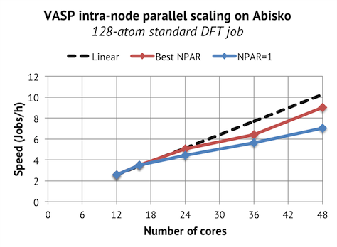
Basically, this is what you get when you ask the queue system for 12,16,24,36,48 cores on 1 node with exclusively running rights (no other jobs on the same node), and you just launch VASP with srun $VASPin the job script. We see that we get nice intra-node scaling. In fact, it is much better than expected, but we will see in the next section that this is an illusion.

The optimal choice of NPARturned out to be:

12 cores NPAR=1
16 cores NPAR=1
24 cores NPAR=3
36 cores NPAR=3
48 cores NPAR=6

This was also surprising, since I had expected NPAR=8 to be optimal. With these settings, there would be MPI process groups of 6 ranks which exactly fit in a NUMA zone. Unexpectedly, NPAR=6 seems optimal when using all 48 cores, and either NPAR=1 or NPAR=3 for the other cases. This does not fit the original hypothesis, but a weakness in our analysis is that we don’t actually know were the processes end up in this scenario, since there is no binding. The only way that you can get a symmetric communication pattern with NPAR=6 is to place ranks in a round robin scheme around each NUMA zone or socket. Perhaps this is what the Linux kernel is doing? An alternative hypothesis is that the unconventional choice of NPAR creates a load imbalance that may actually be beneficial because it allows for better utilization of the second core in each module. To explore this, I decided to test different binding scenarios.

The importance of process binding

To bind MPI processes to a physical core and prevent the operating system from moving them on around inside the compute node, you need to give extra flags to either srun or your MPI launching command such as mpirun. On Abisko, we use srun, where binding is controlled through SLURM by setting e.g. in the job script:

srun --cpu_bind=rank ...

This binds the MPI rank #1 to core #1, and so on in a sequential manner. It is also possible to explicitly specify where each rank should go. The following example binds 24 ranks to alternating cores, so that there is one rank running per Interlagos module:

srun --cpu_bind=map_cpu=0,2,4,6,8,10,12,14,16,18,20,22,24,26,28,30,32,34,36,38,40,42,44,46 ...

In this scheme, neighboring ranks are close to each other: i.e. rank #1 and #2 are in the same NUMA zone. The aim is to maximize the NUMA locality.

The third type of binding I tried was to distribute the ranks in a round-robin scheme in steps of 6 cores. The aim is to minimize NUMA locality, since neighboring ranks are far apart from each other, i.e. rank #1 and #2 are in different NUMA zones.

srun --cpu_bind=map_cpu=0,6,12,18,24,30,36,42,2,8,14,20,26,32,38,44,4,10,16,22,28,34,40,46 ...

Below are the results when comparing the speed of running with 48 cores and 24 cores with different kinds of process binding. The 48 core runs are with NPAR=6 and the 24 cores with NPAR=3.

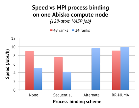
It turns out that you can get all of the performance, and even more, by running with 24 cores in the “fat” mode. The trick is, however, that we need to enable the process binding ourselves. It does not happen by default when you run with half the number of cores per node (the “None” section in the graph).

We can further observe that straight sequential process binding actually worsens performance in the 48 core scenario. Only in the round-robin NUMA scheme (“RR-NUMA”) can we reproduce the performance of the unbound case. This leads me to believe that running with no binding gets you in similar situation with broken NUMA locality, which explains why NPAR=3/6 is optimal, and not NPAR=4.

The most surprising finding,however, is that the top speed was achieved not with the “alternate” binding scheme, which emphasizes NUMA memory locality, but rather with the round-robin scheme, which breaks memory locality of NPAR groups. The difference in speed is small (about 3%), but statistically significant. There are few scenarios where this kind of interleaving over NUMA zones is beneficial, so I suspect that it is not actually a NUMA issue, but rather related to memory caches. The L3 cache is shared between all cores in a NUMA zone, so perhaps the L3 cache is being trashed when all the ranks in an NPAR group are accessing it? It would be interesting to try to measure this effect with hardware counters…

NSIM

Finally, I also made some tests with varying NSIM:

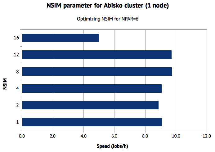
NSIM=4 is the default setting in VASP. It usually gives good performance in many different scenarios. NPAR=4 works on Abisko too, but I gained about 7% by using NPAR=8 or 12. An odd finding was that NPAR=16 completely crippled the performance, doubling the wall time compared to NPAR=4. I have no good explanation, but it obviously seems that one should be careful with too high NPAR values on Abisko.

Conclusion and overall speed

In terms of absolute speed, we can compare with Triolith, where one node with 16 cores can run this example in 380s (9.5 jobs/h) with 512 bands, using the optimal settings of NPAR=2 and NSIM=1. So the overall conclusion is that one Abisko node is roughly 20% faster than one Triolith node. You can easily become disappointed by this when comparing the performance per core, which is 2.5x higher on Triolith, but I think it is not a fair comparison. In reality, the performance difference per FPU is more like 1.3x, and if you compensate for the fact that the Triolith processors in reality run at much higher frequency than the listed 2.2 Ghz, the true difference in efficiency per core-GHz is closer to 1.2x.

Hopefully, I can make some multi-node tests later and determine whether running with 24 cores per node and round-robin binding is the best thing there as well.