

I promised some multi-node scaling tests of the LiFeSiO4 128-atom job in the previous post. Here they come! The choice of NPAR is of particular interest. Do the old rules of NPAR=compute nodesor NPAR=sqrt(number of MPI ranks) still apply here?
To recap: when running on one node, I found that NPAR=3 with 24 cores per compute node and a special MPI process binding scheme (round-robin over NUMA zones) gave the best performance. To check if it still applies across nodes, I ran a full characterization again, but this time with 2 compute nodes. In total, this was 225 calculations!
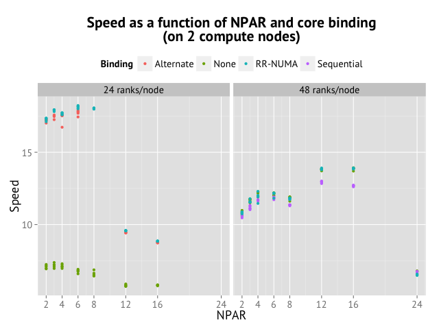
Inspecting the data points shows us that the same approach comes out winning again. Using 24 cores/compute node is still much more effective (+30%) than using all the cores, and NPAR=6 is the best choice. Specifying process binding is essential, but the choice of a particular scheme does not influence as much as in the single node case, presumably because some of the load imbalance now happens in between nodes, which we cannot address this way.
From this I conclude that a reasonable scheme for choosing NPAR indeed seems to be:
NPAR = 3 * compute nodes
Or, if we have a recent version of VASP:
NCORE = 8
The “RR-NUMA” process binding has to be specified explicitly when you start VASP on Abisko:
srun --cpu_bind=map_cpu=0,6,12,18,24,30,36,42,2,8,14,20,26,32,38,44,4,10,16,22,28,34,40,46 /path/to/vasp
When using these settings, the parallel scaling for 1-8 compute nodes looks decent up to 4 compute nodes:
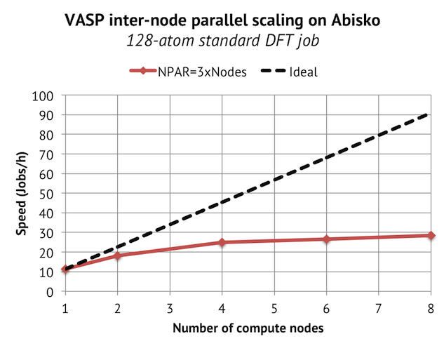
Remember that each node has 48 cores, of which we are using 24 cores, so 4 nodes = 96 MPI ranks. We get a top speed of about 30 Jobs/h. But what does this mean? It seems appropriate to elaborate on the choice of units here, as I have gotten questions about why I measure the speed like this instead of using wall time as a proxy for speed. The reasons is that you could interpret the “Speed” value on the y-axis as the number of geometry optimization steps you could run in one hour of wall time on the cluster. This is something which is directly relevant when doing production calculations.
For reference, we can compare the speeds above with Triolith. On Triolith, the same job (but with 512 bands instead of 480) tops out at about 38 Jobs/h with 16 compute nodes and 256 ranks. So the parallel scaling looks a bit weak compared Triolith, but the absolute time to solution is still good.