Today at Supercomputing 15, the coming release of an official GPU version of VASP 5.4.1 was announced by Nvidia. Both standard DFT and hybrid DFT with Hartree-Fock is GPU accelerated, but there is no GPU-support for GW calculations yet. I have played around with the beta release of GPU-VASP and the speed-up I see when adding 2 K40 GPUs to a dual-socket Sandy Bridge compute node varies between 1.4x to 8.0x, depending on the cell size and the choice of algorithm.
For a long time, VASP was shown in Nvidia’s marketing information as already ported to GPU, despite not being generally available. In fact, I often got questions about it, but had to explain to our users that there were several independently developed prototype versions of VASP with code that had not yet been accepted into the main VASP codebase. But now, an official GPU version is finally happening, and the goal is that it will be generally available to users by the end of the year. No information is available on the VASP home page yet, but I assume that more information will come eventually.
The GPU version is a collaborative effort involving people from several research groups and companies. The list of contributors includes University of Wien, University of Chicago, ENS-Lyon, IFPEN, CMU, RWTH Aachen, ORNL, Materials Design, URCA and NVIDIA. The three key papers, that should be cited when using the GPU version are:
- Speeding up plane-wave electronic-structure calculations using graphics-processing units. Maintz, Eck, Dronskowski. (2011)
- VASP on a GPU: application to exact-exchange calculations of the stability of elemental boron. Hutchinson, Widom. (2011)
- Accelerating VASP Electronic Structure Calculations Using Graphic Processing Units. Hacene, Anciaux-Sedrakian, Rozanska, Klahr, Guignon, Fleurat-Lessard. (2012)
The history of GPU-VASP, as I have understood it, is that after the initial porting work by research groups mentioned above, Nvidia got involved and worked on optimizing the GPU parts, which eventually lead to the acceptance of the GPU code into the main codebase by the VASP developers and subsequently to the launch of the beta testing program coordinated by Nvidia. It is encouraging to see the involvement by Nvidia and I think this is an excellent example of community outreach and industry-academia collaboration. I hope we will see more of this in the future with involvement from other companies. Electronic structure software is, after all, a major workload at many HPC centers. For Intel’s Xeon Phi, VASP is listed as a “work in progress” with involvement from Zuse Institute in Berlin, so we will likely see further vectorization and OpenMP parallelization aimed at manycore architectures as well. I think the fact the GPU version performs as well as it does (see more below) is an indication that there is much potential out there for the CPU version too, in terms of optimization.
Beta-testing GPU-VASP
I have been part of the beta testing program for GPU-VASP. The analysis in this post will approach the subject from two perspectives. The first one is the buyer’s perspective. Does it make economical sense to start looking at GPUs for running VASP? This is the question that we at NSC face as an academic HPC center when we are buying systems for our users. The second perspective is the experience from the user perspective. Does it work? How does it differ from the regular VASP version?
The short answers for the impatient are: 1) possibly, the price/performance might be there given aggressive GPU pricing 2) yes, for a typical DFT calculation, you only need to adjust some parameters in the INCAR file, most importantly NSIM, and then launch VASP as usual.
Hardware setup
The tests were performed on the upcoming GPU partition of NSC’s Triolith system. The compute nodes there have dual-socket Intel Xeon E5-2660 “Sandy Bridge” processors, 64 GB of memory and Nvidia K20 or K40 GPUs. The main difference between the K20 and the K40 is the amount of memory on the card: the K20 has 6 GB and the K40 has 12 GB. VASP uses quite a lot of GPU memory, so with only 6 GB of memory you might see some limitations. For example, the GaAsBi 256 atom test job below used up about 9300 MB per card when running on a single node. It was possible to run smaller jobs on the K20s, though.
I ran most of the tests with the default GPU clock speed of 745 Mhz, but out of curiosity, I also tried to clock up the cards to 875 Mhz with the nvidia-smi utility
$ nvidia-smi -ac 3004,875
It didn’t seem to cause any problems with cooling or stability, and produced a nice 10 % gain in speed. The GPUs are rated for up to 235 Watt, but I never saw them use more than ca 180 W on average during VASP jobs.
Compiling the GPU version
A new build system was introduced with VASP 5.4. When the makefile.include is set up, you can compile the different versions of VASP (regular, gamma-point only, noncollinear) by giving arguments to the make command, e.g.
make std
With GPU-VASP, there is new kind of VASP executable defined in the makefile, called gpu, so the command to compile the GPU version is simply
make gpu
I would recommend sticking to compilation in serial mode. I tried using my old trick of running make -j4 repeatedly to resolve all dependencies, but the new build process does not work as well in parallel, you can get errors during the rsync stages when files are copied between directories.
To compile any program with CUDA, such as GPU-VASP, you need to have the CUDA developer tools installed. They are typically found in /usr/local/cuda-{version} and that is also where you will find them on the Triolith compute nodes. If there are no module files, you can add the relevant directory to your PATH yourself. In this case, CUDA version 7.5:
export PATH=/usr/local/cuda-7.5/bin:$PATH
export LD_LIBRARY_PATH=/usr/local/cuda-7.5/lib64:$LD_LIBRARY_PATH
I tested with CUDA 6.5 in the beginning, and that seemed to work too, but VASP ran significantly faster when I reran the benchmarks with CUDA 7.5 later. Once you have CUDA set up, the critical command to look for is the Nvidia CUDA compiler, called nvcc. The makefiles will use that program to compile and link the CUDA kernels.
$ nvcc --version
nvcc: NVIDIA (R) Cuda compiler driver
Copyright (c) 2005-2015 NVIDIA Corporation
Built on Tue_Aug_11_14:27:32_CDT_2015
Cuda compilation tools, release 7.5, V7.5.17
There is a configuration file for the GPU version in the arch/ directory called makefile.include.linux_intel_cuda which you can use a starting point for configuration. I did not have to make much changes to compile on Triolith. In addition to the standard things like compiler names and flags, one should point out the path to the CUDA tools.
CUDA_ROOT := /usr/local/cuda-7.5
Running
When you log in to a GPU compute node, it is not obvious where to “find” the GPUs and how many there are. There is a utility called nvidia-smi which can be used to inspect the state of the GPUs. Above, I used it for overclocking, but you can also do other things, such as listing the GPUs attached to the system:
[pla@n1593 ~]$ nvidia-smi -L
GPU 0: Tesla K40m (UUID: GPU-f4e02ffa-b01c-1e3e-ebdb-46e1fef83ce6)
GPU 1: Tesla K40m (UUID: GPU-35bee978-8707-1957-12e2-bddda324da88)
And to look at a running job and see how much power and GPU memory that is being used there is nvidia-smi -l
+------------------------------------------------------+
| NVIDIA-SMI 352.39     Driver Version: 352.39         |
|-------------------------------+----------------------+----------------------+
| GPU  Name        Persistence-M| Bus-Id        Disp.A | Volatile Uncorr. ECC |
| Fan  Temp  Perf  Pwr:Usage/Cap|         Memory-Usage | GPU-Util  Compute M. |
|===============================+======================+======================|
|   0  Tesla K40m          Off  | 0000:08:00.0     Off |                    0 |
| N/A   39C    P0   124W / 235W |    558MiB / 11519MiB |     97%      Default |
+-------------------------------+----------------------+----------------------+
|   1  Tesla K40m          Off  | 0000:27:00.0     Off |                    0 |
| N/A   40C    P0   133W / 235W |    558MiB / 11519MiB |     98%      Default |
+-------------------------------+----------------------+----------------------+
The most important thing to make VASP run efficiently is to make sure that you have the MPS system active on the node. MPS is the “Multi Process Service” – it virtualizes the GPU so that many MPI ranks can access the GPU independently without of having to wait for each other. Nvidia has an overview (PDF file) on their web site describing MPS and how set it up. Basically, what you have to do as user is to check if the nvidia-cuda-mps-control process is running. If it is not, you have to start it yourself, before starting your VASP job.
$ mkdir /tmp/nvidia-mps
$ export CUDA_MPS_PIPE_DIRECTORY=/tmp/nvidia-mps
$ mkdir /tmp/nvidia-log
$ export CUDA_MPS_LOG_DIRECTORY=/tmp/nvidia-log
$ nvidia-cuda-mps-control -d
Except for the initialization above, which you only need to do once on the node, you run VASP as usual, using mpiexec.hydra or a similar command, to start an MPI job.
mpiexec.hydra -n 8 vasp_gpu
You should see messages in the beginning of the program output telling you that GPU has been initialized:
Using device 1 (rank 3) : Tesla K40m
Using device 1 (rank 2) : Tesla K40m
Using device 0 (rank 1) : Tesla K40m
Using device 0 (rank 0) : Tesla K40m
running on    4 total cores
distrk:  each k-point on    4 cores,    1 groups
distr:  one band on    1 cores,    4 groups
using from now: INCAR
...
creating 32 CUDA streams...
creating 32 CUFFT plans with grid size 36 x 40 x 48...
(Please note that these might go away or look differently in the final release)
VASP Test Suite
I attempted to run through my VASP test suite with GPU version, but many of the test cases require running with LREAL=.FALSE., so the total energies are different. Despite that, and comparing a few other runs, I did not see any significant discrepancies between the CPU and GPU versions. More than 100 different test cases have been used during the acceptance testing, in addition to the testing done by the beta testers, so we can be certain that the major bugs have been found at this stage.
Performance of standard DFT calculations
I have only performed single-node benchmarks so far, so the focus is comparing the speed when running with CPUs only vs. CPUs+GPUs. The K40 node has 2 GPUs and 2 CPU sockets, with 1 GPU attached to each socket, so the comparison is 16 cores vs (any number of cores) and 2 GPUs. Typically, I found that using 8 MPI ranks (i.e. 8 out of 16 cores on a Triolith node) sharing 2 GPUs using MPS was the fastest combination for regular DFT jobs.
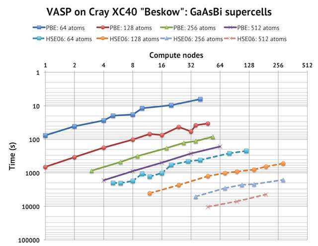
I tested regular DFT by using the old test case of GaAsBi 256 atoms (9 k-points) on which I have collected lots of data on for Triolith (Intel “Sandy Bridge”) and Beskow (Cray XC40 with Intel “Haswell”). As mentioned above, that was close to the biggest job I could run on a single compute node with 2 GPUs due to memory limitations. The reference run with CPUs completed in 7546 seconds on 1 node. With 8 cores and 2 K40 GPUs, it runs remarkably faster and finishes in 1242 seconds, which is around 6 times faster. Here, I used overclocked GPUs (875 Mhz), so at base frequency it is around 10% slower. For reference, with 8 compute nodes using no GPUs, the GaAsBi-256 job completes in 900 seconds on Triolith and in 400 seconds on Beskow.
Interestingly, GPU-VASP is especially strong on the Davidson algorithm. ALGO=fast runs about 50% faster in CPU mode, but with GPUs, there is very little difference, so if you rely on ALGO=normal for getting convergence, there is good news. If you calculate the speed-up for ALGO=normal, it is therefore higher, around 8x faster.
The NSIM parameter is now very important for performance. Theoretically, the GPU calculations will run faster the higher the value of NSIM you set, with the drawback being that the memory consumption on the GPUs increase with higher NSIM as well. The recommendation from the developers is that you should increase NSIM as much you can until you run out of memory. This can require some experimentation, where you have to launch your VASP job and the follow the memory use with the nvidia-smi -l command. I generally had to stop at NSIM values of 16-32.
Packing a relatively big cell like this (256 atoms) on a single node is probably the poster case for the GPU version, as you need sufficiently large chunks of work offloaded onto the GPU in order to account for the overhead of sending data back and forth between the main memory and the GPU. As an example of what happens when there is too little work to parallelize, we can consider the 128-atom Li2FeSiO4 test case in the gamma point only. I can run that one on a CPU node with the gamma point version of VASP in around 260 seconds. The GPU version, which has no gamma point optimizations, clocks in 185 seconds, even with 2 K40s GPUs, for an effective improvement of only 40%.
Of course, one can argue that this is an apples to oranges comparison, and that you should compare with the slower VASP NGZhalf runtime for the CPU-version (which is 428 seconds or half the speed of the GPU run), but the gamma-point only optimization is available in the CPU version today, and my personal opinion is that the symmetries enforced in the gamma point version produces more accurate results, even if they might be different.
Performance of hybrid DFT calculations
Hybrid DFT calculation incorporating Hartree-Fock, perhaps screened such as in HSE06, are becoming close to the standard nowadays, as regular DFT is no longer considered state of the art. Part of the reason is the availability of more computing resources, as an HSE06 calculation can easily take 100 times longer to run. Speeding up hybrid calculation was one of the original motivations for GPU-accelerating VASP, so I was curious to test this out. Unfortunately, I had lots of problems with memory leaks and crashes in the early beta versions, so I had a hard time getting any interesting test cases to run. Eventually, though, these bugs were ironed out in the last beta release, enabling me to start testing HSE06 calculations, but the findings here should be considered preliminary for now.
In my tests, I found that 4-8 MPI ranks was optimal for hybrid DFT. The reason for hybrid jobs being able to get along with less CPU cores is that the Hartree-Fock part is the dominant part, and it runs completely on the GPU, so there should be some efficiency gain by having less MPI ranks competing for the GPU resources. For really big jobs, I was told by Maxwell Hutchinson, one of the exact-exchange GPU developers, that having 1 GPU per MPI rank should be the best way to run, but I have not been able to confirm that yet.
Setting NSIM is even more important here, the recommendation is
NSIM = NBANDS / (2*cores)
So you need to have lots of bands in order to fully utilize the GPUs.
The test case here was an MgO cell with 63 atoms, 192 bands and 4 k-points. These are quite heavy calculations so I had to resort to timing individual SCF iterations to get some results quickly. With 16 CPU cores only, using ALGO=all one SCF iteration requires around 900 seconds. When switching to 4 cores and 2 GPU:s (2 cores per GPU), I get the time for one SCF iteration down to around 640 seconds, which is faster, but not a spectacular improvement (40-50%). But note that the same SCF algorithm is not being used here, so actual number of iterations required to converge might be different, which affects the total runtime. I have actually not tested running HSE06 calculations with ALGO=normal before, as it is not the standard way to run, so I cannot say right now whether to expect faster convergence with ALGO=normal. The underlying problem, as I have understood it, is that a job like this launches lots of small CUDA kernels, and although there are many of them, they cannot effectively saturate the GPU. The situation should be better for larger cells, but I have not been able to run these test yet, as I only had a few nodes to play with.
Summary and reflections
It is well known that making a fair comparison between CPU and GPU computing is very challenging. The conclusion you come to is to a large extent dependent on which question you ask and what you are measuring. The whole issue is also complicated by the fact that many of the improvements made to the code during the GPU porting can be back-ported to the CPU version, so the process of porting a code to GPU might itself, paradoxically, weaken the (economical) case for running on GPUs, as the associated gain might make the CPU performance just good enough to compete with GPUs.
From a price/performance point of view, one should remember that a GPU-equipped node is likely to be much more expensive and use more power when running. In a big procurement of an HPC resource, the final pricing is always subject to some negotiation and discounting, but if one looks at the list prices, a standard 2-socket compute node with 2 K40 GPUs is likely to cost at least 2-3 times as much as without the GPUs. One must also take into consideration that such a GPU node might not always run GPU-accelerated codes and/or be idling some part of the time due to a lack of appropriate jobs. Consequently, the average GPU workload that runs on a GPU partition in an HPC cluster must run a lot faster to make up for the higher cost. In practice, a 2-3x speedup for a breakeven with respect to pricing is probably not enough to make it economically viable, instead we are looking at maybe 4-6x. The good news is, of course, that certain VASP workloads (such as normal DFT and molecular dynamics on big cells) do meet this requirement.
Another perspective that should not be forgotten is that the compute power of a single workstation running VASP can be improved a lot with GPUs. This is perhaps not as relevant for “big” HPC, but it significantly increases the total compute power and job capacity that a VASP user without HPC access can easily acquire. From a maintenance and system administration perspective, there is a big jump in moving from a single workstation to a full-fledged multi-node cluster. A cluster needs rack space, a queue system, some kind of shared storage etc. The typical scientist, will not be able to set up such a system easily. The 2-socket workstation of yesterday was probably not sufficient for state of the art VASP calculations, but with, let us say, an average 4x improvement with GPUs, it might be viable for certain kinds of research level calculations.
From a user and scientific point of view, the GPU version of VASP seems ready for wider adoption. It works and is able to reproduce the output of the regular VASP. Running it requires making some change of settings in the input files, which unfortunately can make the job suboptimal when running on CPUs. But it has always been the case, that you need to adjust the INCAR parameters to get the best out of a parallel run, so that is nothing new.
In conclusion, it would not surprise me if the availability of VASP with CUDA support might be a watershed event for the adoption of Nvidia’s GPUs, since VASP is such a big workload on many HPC centers around the world. For us, for example, it has definitely made us consider GPUs for the next generation cluster that will eventually replace Triolith.
P.S. 2015-11-23: The talk by Max Hutchinson at SC15 about VASP for GPU is now available online.
]]>