Atomic Simulation Environment on Triolith

Yesterday, I installed a new version of the Atomic Simulation Environment on Triolith. ASE allows you to script your ab initio calculations using Python. Here comes a tutorial on how you can run VASP calculations with ASE on Triolith. It is a little bit more elaborate than the official documentation of VASP module which can be found on the ASE web site.

First, we need to load the Python and ASE modules. I recommend the python/2.7.4-snic-1 module.

module load python/2.7.4-snic-1 ase/3.7.1

Next, we need to tell ASE’s VASP module where to find the VASP binaries and the POTCARs files.

export VASP_COMMAND="mpprun /software/apps/vasp/5.3.3-18Dec12/default/vasp"
export VASP_PP_PATH=/software/apps/vasp/POTCARs

Note that ASE requires that there are directories called potpaw, potpaw_GGA and potpaw_PBE below the VASP_PP_PATH, so you may have to create symlinks with these names if you don’t have them in your own database.

Now, we need to create the actual ASE Python script that sets up the calculation. The idea in this little example is to calculate the equilibrium volume and bulk modulus of hcp Mg.

(mg-hcp.py) download
1
2
3
4
5
6
7
8
9
10
11
12
13
14
15
16
17
18
19
20
21
22
23
24
25
26
27
28
29
30
31
32
33
34
35
36
37
38
39
40
41
42
43
44
45
46
47
48
49
import numpy
from ase.structure import bulk
from ase.calculators.vasp import Vasp
from ase.units import GPa
from ase.utils.eos import EquationOfState

jobs = []

# Generate cell configurations
for volume in numpy.linspace(0.90,1.10,10):
  mg = bulk('Mg','hcp',a=3.1,covera=1.62)
  mg.set_cell(mg.get_cell()*volume,scale_atoms=True)

  calc = Vasp(prec = 'Accurate',
            xc = 'PBE',
            lreal = False,
            encut = 150.0,
            istart =0,
            icharg= 2,
            nelm = 20,
            kpts = [6,6,6],
            ismear = 1,
            sigma = 0.2,
            algo = "fast")

  mg.set_calculator(calc)

  jobs.append(mg)

# Run jobs
volumes = [job.get_volume() for job in jobs]
energies = [job.get_potential_energy() for job in jobs]

print "Calculation output"
print "------------------"
print "Volumes:", volumes
print "Energies:", energies
print

# Fit EOS
eos = EquationOfState(volumes,energies)

v0,e0,B = eos.fit()

print "Equation of state parameters"
print "----------------------------"
print "E0: %2.6f eV" % (e0)
print "V0: %2.1f A^3" % (v0)
print "B: %2.1f GPa" % (B/GPa)

The script works like this: first, we create cells for 10 different volumes and at the same time attach VASP settings to them, then we call get_potential_energy() for each of these cells and collect the energies and volumes, and finally, we use ASE’s built-in equation of state subroutine to calculate the equilibrium volume and bulk modulus.

To run this script on a Triolith compute node, we need to create a job script. In the job script, we just launch the Python script, which will start ASE and then launch VASP for us.

#!/bin/bash
#SBATCH -J mg 
#SBATCH -N 1
#SBATCH --exclusive
#SBATCH -t 0:10:00

python mg-hcp.py

Submit by sbatchas usual.

sbatch mg.sh

When the job has completed (it should not take more than a few minutes), look in the slurm.out file for the output from ASE.

[pla@triolith1 asetest]$ cat slurm-693921.out 
Calculation output
------------------
Volumes: [30.469003876435877, 32.782153276649034, 35.209509626875203, 37.753824901813466, 40.417851076162975, 43.204340124622782, 46.116044021892051, 49.155714742669836, 52.326104261655324, 55.629964553547552]
Energies: [-1.86460718, -2.2747034, -2.5757448, -2.78654685, -2.92182549, -2.99416931, -3.01374966, -2.99022215, -2.93151648, -2.84418079]

Equation of state parameters
----------------------------
E0: -3.013844 eV
V0: 45.9 A^3
B: 36.5 GPa

The experimental bulk modulus of Mg is ca 45 GPa, so the result seems reasonable.

Compiling VASP With Gfortran

For some time, VASP has been centered on the x86 processors and Intel’s Fortran compiler. Inside the VASP source distribution, you can find some makefiles for other compilers, but they seldom work nowadays, and in many cases you need to make modifications to the source code to make it work with other compilers.

In particular, recent versions of Gfortran cannot compile VASP. If you try, the compiler would stop at errors concerning a circular dependency of a module (i.e. the module includes itself), and some output formatting errors.

From what I can understand, these problems are actually related to violations of the Fortran language standard, which are allowed by the Intel compiler. There are no compiler flags for gfortran that let you “relax” the standard like this to let it compile VASP, so you need to modify the source to make it compliant.

When I tested with gcc 4.7.2 and gcc 4.8.0, four files needed to be modified: us.F, vdwforcefield.F, finite_diff.F, and spinsym.F. I have prepared the patches as a “patch file” which you can download. To apply the patches to the source code, locate your VASP 5.3.3 source code directory and do

cd vasp.5.3
patch -p0 < vasp533gcc.patch

In the makefile, you need to set the following compiler flags for gfortran.

FC = mpif90 (or similar depending on the MPI)
FFLAGS = -ffree-form -ffree-line-length-0  -fno-second-underscore
OFLAG=-O3 -march=corei7-avx -mtune=corei7-avx

Global -O3 optimization seems to work for me on Triolith (Xeon E5 processors), but I haven’t tested all functionality of the gfortran version yet. As with the Intel compiler, you may have to decrease the optimization or disable aggressive inlining in certain files.

In the preprocessor section, put something like this. Note that you should not use the -DPGF90 flag when compiling with gfortran.

CPP     = $(CPP_)  -DHOST=\"NSC-GFORTRAN-B01\" -DMPI 
    -DMPI_BLOCK=262144 \
    -Duse_collective -DCACHE_SIZE=12000 -Davoidalloc -DNGZhalf\

These tricks made it for me, and I now have a reference version of VASP compiled with Gfortran on Triolith. The speed seems to be about same as when compiled with Intel Fortran, since VASP relies heavily on FFTWs and BLAS calls and I still link with MKL and Intel’s MPI.

Later, I will try to make a longer guide how to compile VASP with a fully free software stack, and compare performance and stability.

Scaling of Small Jobs on the Abisko Interlagos Cluster

I promised some multi-node scaling tests of the LiFeSiO4 128-atom job in the previous post. Here they come! The choice of NPAR is of particular interest. Do the old rules of NPAR=compute nodesor NPAR=sqrt(number of MPI ranks) still apply here?

To recap: when running on one node, I found that NPAR=3 with 24 cores per compute node and a special MPI process binding scheme (round-robin over NUMA zones) gave the best performance. To check if it still applies across nodes, I ran a full characterization again, but this time with 2 compute nodes. In total, this was 225 calculations!

Speed of VASP on Abisko as a function NPAR and binding

Inspecting the data points shows us that the same approach comes out winning again. Using 24 cores/compute node is still much more effective (+30%) than using all the cores, and NPAR=6 is the best choice. Specifying process binding is essential, but the choice of a particular scheme does not influence as much as in the single node case, presumably because some of the load imbalance now happens in between nodes, which we cannot address this way.

From this I conclude that a reasonable scheme for choosing NPAR indeed seems to be:

NPAR = 3 * compute nodes

Or, if we have a recent version of VASP:

NCORE = 8

The “RR-NUMA” process binding has to be specified explicitly when you start VASP on Abisko:

srun --cpu_bind=map_cpu=0,6,12,18,24,30,36,42,2,8,14,20,26,32,38,44,4,10,16,22,28,34,40,46 /path/to/vasp

When using these settings, the parallel scaling for 1-8 compute nodes looks decent up to 4 compute nodes:

Inter-node scaling on Abisko

Remember that each node has 48 cores, of which we are using 24 cores, so 4 nodes = 96 MPI ranks. We get a top speed of about 30 Jobs/h. But what does this mean? It seems appropriate to elaborate on the choice of units here, as I have gotten questions about why I measure the speed like this instead of using wall time as a proxy for speed. The reasons is that you could interpret the “Speed” value on the y-axis as the number of geometry optimization steps you could run in one hour of wall time on the cluster. This is something which is directly relevant when doing production calculations.

For reference, we can compare the speeds above with Triolith. On Triolith, the same job (but with 512 bands instead of 480) tops out at about 38 Jobs/h with 16 compute nodes and 256 ranks. So the parallel scaling looks a bit weak compared Triolith, but the absolute time to solution is still good.

VASP on the Abisko Cluster (With AMD Interlagos)

When Triolith had a service stop recently, I took to the opportunity to explore the Abisko cluster at HPC2N in Umeå. Abisko has 4-socket nodes with 12-core AMD Opteron “Interlagos” processors and lots of memory. Each compute node on Abisko features an impressive 500 gigaflop/s theoretical compute capability (compared to e.g. Triolith’s Xeon E5 nodes with 280 gigaflop/s). The question is how much of this performance we can get in practice when running VASP and how to set important parallelization parameters such as NPAR and NSIM.

Summary of findings

  • One Abisko node is about 20% faster than one Triolith node, but you have to use 50% more cores and twice the memory bandwidth to get the job done.
  • You should run with 24 cores per node. More specifically, one core per Interlagos “module”.
  • It is imperative that you specify MPI process binding explicitly either with mpirun or srun to get good speed.
  • Surprisingly, process binding in a round-robin scheme over NUMA zones is preferable to straight sequential binding of 1 rank per module. (Please see below for the binding masks I used)
  • NPAR: MPI ranks should be in groups of 8, this means NPAR=3*nodes.
  • NSIM: 8, brings you +10% performance vs the default choice.

Background on AMD Interlagos

To understand the results, we first need to have some background knowledge about the Interlagos processors and how they differ from earlier models.

The first aspect is the number of cores vs the number of floating-point units (FPU:s). The processors in Abisko are marketed by AMD as having 12 cores, but in reality there are only 6 FPU:s, each which are shared between 2 cores (called a “module”). So I consider them more like 6-core processors capable of running in two modes: either a “fat mode” with 1 thread with 8 flops/cycle or a “thin mode” with 2 threads with 4 flops/cycle. Which one is better will depend on the mix of integer and floating point instructions. In a code like VASP, which is heavily dependent on floating point calculations and memory bandwidth, I would expect that running with 6 threads is better because there is always some overhead involved with using more threads.

The second aspect to be aware of is the memory topology. Each node on Abisko has 48 cores, but they are separated into 8 groups, each of which have their own local memory. Each core can still access memory from everywhere, but it is much slower to read and write memory from a distant group. These groups are usually called NUMA zones (or nodes, or islands). We would expect that we need to group the MPI processes by tweaking the NPAR parameter to reflect the NUMA zone configuration. Specifically, this means 8 groups of 6 MPI ranks per compute node on Abisko, but more about that later.

Test setup

Here, we will be looking at the Li2FeSiO4 supercell test case with 128 atoms. I am running a standard spin-polarized DFT calculation (no hybrid), which I run to self-consistency with ALGO=fast. I adjusted the number of bands to 480 to better match the number of cores per node.

Naive single node test

A first (naive) test is to characterize the parallel scaling in a single compute node, without doing anything special such as process binding. This produced an intra-node scaling that looks like this after having tuned the NPAR values:

Intra-node scaling on Abisko

Basically, this is what you get when you ask the queue system for 12,16,24,36,48 cores on 1 node with exclusively running rights (no other jobs on the same node), and you just launch VASP with srun $VASPin the job script. We see that we get nice intra-node scaling. In fact, it is much better than expected, but we will see in the next section that this is an illusion.

The optimal choice of NPARturned out to be:

12 cores NPAR=1
16 cores NPAR=1
24 cores NPAR=3
36 cores NPAR=3
48 cores NPAR=6

This was also surprising, since I had expected NPAR=8 to be optimal. With these settings, there would be MPI process groups of 6 ranks which exactly fit in a NUMA zone. Unexpectedly, NPAR=6 seems optimal when using all 48 cores, and either NPAR=1 or NPAR=3 for the other cases. This does not fit the original hypothesis, but a weakness in our analysis is that we don’t actually know were the processes end up in this scenario, since there is no binding. The only way that you can get a symmetric communication pattern with NPAR=6 is to place ranks in a round robin scheme around each NUMA zone or socket. Perhaps this is what the Linux kernel is doing? An alternative hypothesis is that the unconventional choice of NPAR creates a load imbalance that may actually be beneficial because it allows for better utilization of the second core in each module. To explore this, I decided to test different binding scenarios.

The importance of process binding

To bind MPI processes to a physical core and prevent the operating system from moving them on around inside the compute node, you need to give extra flags to either srun or your MPI launching command such as mpirun. On Abisko, we use srun, where binding is controlled through SLURM by setting e.g. in the job script:

srun --cpu_bind=rank ...

This binds the MPI rank #1 to core #1, and so on in a sequential manner. It is also possible to explicitly specify where each rank should go. The following example binds 24 ranks to alternating cores, so that there is one rank running per Interlagos module:

srun --cpu_bind=map_cpu=0,2,4,6,8,10,12,14,16,18,20,22,24,26,28,30,32,34,36,38,40,42,44,46 ...

In this scheme, neighboring ranks are close to each other: i.e. rank #1 and #2 are in the same NUMA zone. The aim is to maximize the NUMA locality.

The third type of binding I tried was to distribute the ranks in a round-robin scheme in steps of 6 cores. The aim is to minimize NUMA locality, since neighboring ranks are far apart from each other, i.e. rank #1 and #2 are in different NUMA zones.

srun --cpu_bind=map_cpu=0,6,12,18,24,30,36,42,2,8,14,20,26,32,38,44,4,10,16,22,28,34,40,46 ...

Below are the results when comparing the speed of running with 48 cores and 24 cores with different kinds of process binding. The 48 core runs are with NPAR=6 and the 24 cores with NPAR=3.

Speed vs process binding on Abisko

It turns out that you can get all of the performance, and even more, by running with 24 cores in the “fat” mode. The trick is, however, that we need to enable the process binding ourselves. It does not happen by default when you run with half the number of cores per node (the “None” section in the graph).

We can further observe that straight sequential process binding actually worsens performance in the 48 core scenario. Only in the round-robin NUMA scheme (“RR-NUMA”) can we reproduce the performance of the unbound case. This leads me to believe that running with no binding gets you in similar situation with broken NUMA locality, which explains why NPAR=3/6 is optimal, and not NPAR=4.

The most surprising finding,however, is that the top speed was achieved not with the “alternate” binding scheme, which emphasizes NUMA memory locality, but rather with the round-robin scheme, which breaks memory locality of NPAR groups. The difference in speed is small (about 3%), but statistically significant. There are few scenarios where this kind of interleaving over NUMA zones is beneficial, so I suspect that it is not actually a NUMA issue, but rather related to memory caches. The L3 cache is shared between all cores in a NUMA zone, so perhaps the L3 cache is being trashed when all the ranks in an NPAR group are accessing it? It would be interesting to try to measure this effect with hardware counters…

NSIM

Finally, I also made some tests with varying NSIM:

“Speed

NSIM=4 is the default setting in VASP. It usually gives good performance in many different scenarios. NPAR=4 works on Abisko too, but I gained about 7% by using NPAR=8 or 12. An odd finding was that NPAR=16 completely crippled the performance, doubling the wall time compared to NPAR=4. I have no good explanation, but it obviously seems that one should be careful with too high NPAR values on Abisko.

Conclusion and overall speed

In terms of absolute speed, we can compare with Triolith, where one node with 16 cores can run this example in 380s (9.5 jobs/h) with 512 bands, using the optimal settings of NPAR=2 and NSIM=1. So the overall conclusion is that one Abisko node is roughly 20% faster than one Triolith node. You can easily become disappointed by this when comparing the performance per core, which is 2.5x higher on Triolith, but I think it is not a fair comparison. In reality, the performance difference per FPU is more like 1.3x, and if you compensate for the fact that the Triolith processors in reality run at much higher frequency than the listed 2.2 Ghz, the true difference in efficiency per core-GHz is closer to 1.2x.

Hopefully, I can make some multi-node tests later and determine whether running with 24 cores per node and round-robin binding is the best thing there as well.

Making Supercells for VASP

I often get questions on how to make supercells for VASP calculations. The problem is typically that you have a structure in a POSCAR file and then want to expand it to a bigger supercell to study e.g. defects. There are many programs available that can perform this task, like PHON and Phonopy, and if you google, you can find many scripts, usually called “vasputil” that can do this task specifically. Many people in your research group have probably written their own program as well.

What I really recommend, however, is to not reinvent the wheel and instead use already available libraries to analyze and work with your ab initio calculations. One such library is the Atomic Simulation Environment (ASE) for Python, which supports many programs, including VASP. With ASE, you can do really cool stuff like making small Python programs which read your VASP input/output and then work on them programmatically. In fact, with ASE, it is almost trivial to make supercells. You can do it with 3 lines of Python code:

import ase.io.vasp
cell = ase.io.vasp.read_vasp("POSCAR")
ase.io.vasp.write_vasp("POSCAR.4x4x4",cell*(4,4,4), label='444supercell',direct=True,sort=True)

The code above reads a POSCAR file in the current working directory, transforms it to a 4x4x4 supercell and writes the results to disk as “POSCAR.4x4x4”. Note that to run this on Triolith, you need to have the ASE module loaded

module load ase/3.6.0

I thought this trick might be useful, so I made a script that can perform this procedure available in the vasptools module on Triolith. The script is called supersize and takes a POSCAR file as the first argument, and the supercell sizing as the second:

$ supersize POSCAR 4x4x4

The output is a new POSCAR file called “POSCAR.4x4x4” containing the supercell repeated 4 times in a,b,c directions.

Quantum Espresso vs VASP (Round 2)

In the second round, I wanted to do a medium-sized, more complicated system. The original plan was to run the Li2FeSiO4 supercell with spin polarization, which I have run extensively in VASP before. It is a nontrivial example from my previous research, and it can be tricky to get fast convergence to the right ground state. Unfortunately, I failed at getting the Li2FeSiO4 system to run. PWscf kept crashing, despite much tinkering, and all I got was the following error message:

Error in routine rdiaghg (1539): S matrix not positive definite

The QE documentation does mention these kinds of errors saying that they are related to negative charges densities in the cores, which is basically either due to an unreasonable crystal structure or a poor choice of pseudopotentials. Standard tricks like increasing the encutrho parameter or changing the diagonalization algorithm did not help either, so my guess is that something was wrong with the available PAW datasets. The all-electron Li PAW, for example, comes with a suggested plane wave cutoff of 1100 eV, unlike 272 eV in VASP. I am not sure if it is numerically sane to mix it with the other ones with much lower cutoff. I have seen this give rise to numerical instabilities in VASP, for example.

New test case: Fe-N-doped graphene

Instead, I constructed a 128-atom supercell of graphene. I inserted an Fe cation site coordinated by four pyridinic sites, to make it a little bit more exciting and also have a reason to do spin polarization.

N-Fe-doped graphene

The PAW datasets were:

Fe.pbe-spn-kjpaw_psl.0.2.1.UPF (16 valence)
C.pbe-n-kjpaw_psl.0.1.UPF (4 valence)
N.pbe-n-kjpaw_psl.0.1.UPF (5 valence)

In total, this system has 127 atoms and 524 electrons, so 512 bands per spin channel is a nice and even number here. There is a similar issue with plane-wave cutoff as in the previous example. I set it to 500 eV to compare with the VASP calculation. It could be argued that it is artificially low, and that a real production calculation with QE using the PAW potentials would need to have a bigger cutoff.

A 500 eV basis requires an FFT grid of 144x144x72 points, which in the case of VASP means that an optimal plan-wise decomposition of the FFTs can be achieved for 1,2,4,8, and 12 compute nodes by using NPAR=1,2,4,8,12, respectively. If I understand the PWscf documentation correctly, 72 FFT planes in Z-direction means that we should be able to scale up to 2x72 MPI ranks, since we have spin polarization (2 “effective” k-points), and that we are also likely to be helped by FFT task group parallelization using the -ntg command line flag.

I ran the jobs on 1,2,4,8,12, and 16 Triolith compute nodes, using all available cores (16 cores per node). For VASP, the optimal setting is band parallelization using NPAR=compute nodes, and LPLANE=.TRUE.. All PWscf calculations were run with -npool 2, which activates k-point parallelization, together with several combinations of -ntg and -ndiag, which controls FFT task parallelization and SCALAPACK linear algebra parallelization. There is experimental support for band parallelization in QE (-nband flag), but it either crashed the program or ran horribly slow, so the results below are using the standard parallelization options.

Results

Fe-N-doped graphene QE vs VASP speed

VASP scales acceptably up to 12 nodes / 192 cores, whereas QE only has decent scaling from 1 to 2 nodes. I believe that the reason is that VASP has band parallelization, but QE not. To test my theory, I ran the VASP jobs with as low NPAR as possible, which is shown as the blue dotted line. This meant NPAR=1 (no band parallelization) for 1-8 nodes, and NPAR=2 for 12-16 nodes. The parallel scaling is much worse then, and essentially flat from 8 nodes and upwards, which is similar to the QE results.

In terms of absolute performance, VASP and QE are tied again when running on 16 and 32 cores, with PWscf actually being about 10% faster on 32 cores. But when comparing the top speed, VASP achieves at least 25 Jobs/h with 16 nodes vs. 10 Jobs/h with PWscf on 8 nodes. So we are looking at half the time to solution with VASP.

Another purpose of this study was to characterize the parallelization settings for QE when running on Triolith. The best parallelization settings for this system turned out to be:

Nodes -ntg  -ndiag
1        1      16
2        1      16
4        2      16
8        2      16
12       4      16
16       4      16

FFT task groups (-ntg) seems to be necessary for higher core counts, just as suggested in the QE manual. The rule of thumb in the manual is to enable -ntg when the number of cores exceeds the number of FFT mesh points in the z direction, which seems accurate in this case.

I found the performance curve for SCALAPACK parallelization very flat for ndiag=16/25/36, so I was unable to resolve any difference with just 3-5 samples per point, but it seems like the performance flattens out above 16 cores for this system. Diagonalizing a 512x512 matrix is not that big of a task in the context of SCALAPACK, so this is not surprising.

Mixing and SCF stability turned out to be an influential factor when making the comparison between VASP and PWscf. The default mixing scheme in VASP is very good and can converge the graphene system studied here in ca 32 SCF iterations using default settings, but getting down to that level with PWscf required tuning of beta (0.2) and change of the mixing mode from plain to local-TF.

Conclusion

When it comes to bigger, more realistic calculations, PWscf is not as straightforward to work with as VASP. This is a combination of the robustness and availability of PAW datasets, and the increased need of parameter tuning necessary to get decent performance. The speed is on par with VASP for 1-2 compute nodes, but VASP has a much faster and more predictable parallel scaling beyond that. It was a surprise to me to not find working band parallelization in PWscf.

Quantum Espresso vs VASP (Round 1)

There are just a few implementations of the PAW method: PWPAW, ABINIT, VASP, GPAW, and in the PWscf program in Quantum Espresso (“QE” from now on). VASP is frequently held up as the fastest implementation, and I concluded in earlier tests that standard DFT in ABINIT is too slow compared to VASP to be useful for when running large supercells. But how does QE compare to VASP? There has been extensive work on QE in the last years, such as adding GPU support and mixed OpenMP/MPI parallelism, and you can find papers showing good parallel scalability such as (ref1) and (ref2). By request, I will therefore perform and publish some comparisons of VASP and QE, in the context of PAW calculations. Primarily, I am interesting in:

  • Raw speed, measured as performance on a single 16 core compute node.
  • Parallel scalability, measured as the time to solution and computational efficiency for very large supercell calculations.
  • General robustness and production readiness, in particular numerical stability, sane defaults, and quality of documentation.

So as the first step, before going into parallel scaling studies, it is useful to know the performance on the level of a single compute node. In the ABINIT vs VASP study, I used a silicon supercell with 31 atoms and one vacancy for basic testing. I will use it here as well to provide a point of reference.

Methods

Access to prepared PAW dataset is crucial for a PAW code to be useful, as most users prefer to not generate pseudopotentials themselves (although it can be discussed whether this is a wise approach). Fortunately, there are now more PAW datasets available for QE. I found “Si.pbe-n-kjpaw_psl.0.1.UPF” to be the most similar one to VASP’s standard silicon POTCAR. It is a scalar relativistic setup with 4 valance electrons for the PBE exchange-correlation functional. It differs in the suggested plane-wave cutoff, though, where the QE value is much higher (13.8 Ry, ca 500 eV) compared to the VASP one (250 eV). I decided to use 250 eV in both programs for benchmarking purposes, but it is a highly relevant question if you get the same physical results at this cutoff? I will postpone the discussion of differences between PAW potentials for now, but I expect to return to it at a later time.

As usual, I put some effort into making sure that I am running as similar calculations as possible from a numerical point of view:

  • The plane-wave cutoff was set to 18.4 Ry/250 eV. This lead to a 72x72x72 coarse FFT grid in both programs.
  • The fine FFT grids were 144x144x144.
  • 80 bands, set manually
  • 6 k-points (automatically generated)
  • 6 symmetry operations detected in the crystal lattice
  • SCF convergence thresholds were 1.0e-6 Ry and 1.0e-5 eV, respectively.
  • Minimal disk I/O (i.e. no writing of WAVECAR and wfc files).

A notable difference is that PWscf does not have the RMM-DIIS algorithm, instead I used the default Davidson iterative diagonalization. In the VASP calculations, I used the hybrid Davidson/RMM-DIIS approach (ALGO=fast), which is what I would use in a real-life scenario.

VASP was compiled with the -DNGZhalf preprocessor option for improved FFT performance. I could not find a clear answer in the PWscf documentation about this feature, but it does use the real FFT representation for gamma point calculations, so I presume that the “half” representation is also employed for normal calculations.

Results

Results when running the Si 31 atom cell on 1 Triolith compute node (16 Xeon E5 cores clocked at 2.2-3.0 Ghz):

Si31 cell QE vs VASP speed

It is great to find VASP and QE pretty much tied for this test case. VASP is around 6% faster, but the QE calculation also required 20 SCF steps instead of 15 steps in VASP, so it is possible that a more experienced QE user would be able to tune the SCF convergence better to achieve at least parity in speed.

I ran with both 8 cores and 16 cores per node to get a feel for the intra-node parallel scaling. QE actually scales better with 1.6x speed-up from 8 to 16 cores, vs 1.3x for VASP. This indicates to me that QE puts less pressure on the memory system and could scale better on big multicore nodes.

I also tested the OpenMP enabled version of QE, but for this test case there was no real benefit in terms of speed: 8 MPI ranks with 2 OpenMP threads each did run faster (+27%) than 8 ranks with only MPI, but not as fast as with 16 MPI ranks. But there was a slight reduction in memory: 16 MPI ranks with -npool 2 required a maximum of 678 MB of memory, whereas 8 MPI ranks with 2 OpenMP threads used only 605 MB. So by using this approach, you could save some memory at the expense of speed. VASP, for comparison, used 1205 MB with k-point parallelization with 16 ranks, but 706 MB with band parallelization (which was the fastest option), so the memory usage of QE and VASP is very similar in practice.

Summary

In conclusion, this was my first serious calculations with PWscf and my overall impression is that the PAW speed is promising, and that it was relatively painless to set up the calculation and get going. I found the documentation comprehensive, but somewhat lacking in organization and mostly of reference kind. There are no explicit examples or practical notes of what you actually need to do to run a typical calculation. In fact, in my first attempt, I completely failed at getting PWscf to read my input files — I had to consult with an experienced QE user to understand why QE would not read my atomic positions (it turned out that the ATOMIC_POSITIONS section is only read if “nat” is set in the SYSTEM section). Once over the initial hurdle, it was a quite smooth ride, though. SCF convergence was achieved using the default settings, and all symmetries were detected correctly: that is something you cannot take for granted in all electronic structure codes.

Next up is a medium-sized calculation, the Li2FeSiO4 supercell with 128 atoms.

Tuning VASP: BLAS and FFT on Cray XE6

I did some more testing of BLAS and FFT libraries for VASP on Cray XE6, while working on VASP 5.3.3 for PDC’s Lindgren. Before, I always prepared VASP with Intel MKL and Cray MPI. This was mostly for compatibility reasons, but benchmarking also showed that the MKL version was much faster (ca 10%-20%) than the LibSci version. It is counterintuitive, since Cray has optimized BLAS routines in LibSci (in addition to the standard ones from GotoBLAS). Why was MKL so much faster? Could it be the FFT subroutines, just like what I saw on Sandy Bridge cpu:s? I decided to build a version of VASP with BLAS/LAPACK from LibSci and FFTs from Intel’s MKL to test this hypothesis. For reference, the LibSci version was 11.1, and the MKL version the one included in PrgEnv-intel/4.0.46, i.e. 10.3.

Speed Cray LibSci vs MKL

I ran three test systems:

  • Li2FeSiO4 cell with 128 atoms, standard DFT, with 2 compute nodes.
  • MgO cell with 63 atoms using HSE06 and k-point parallelization over 3 compute nodes.
  • NiSi cell with 504 atoms over 16 compute nodes (384 cores), standard DFT.

The MKL version is indeed faster than the LibSci version, +7-12%, but it is possible to squeeze out a few % more performance by combining LibSci with MKL. The system jitter on Lindgren is normally very low , so the differences here are statistically significant. So, for the 5.3.3 version, I decided to deploy the LibSci+MKL version on Lindgren.

How to Compile VASP on Cray XE6

Here are some instructions for making a basic installation of VASP 5.3.3 on Cray XE6. It applies specifically to the Cray XE6 at PDC called “Lindgren”, but Cray has a similar environment on all machines, so it might be helpful for other Cray sites as well.

First, download the prerequisite source tarballs from the VASP home page:

http://www.vasp.at/ 

You need both the regular VASP source code, and the supporting “vasp 5” library:

vasp.5.3.3.tar.gz
vasp.5.lib.tar.gz

I suggest to make a new directory called e.g. vasp.5.3.3, where you download and expand them. You would type commands approximately like this:

mkdir 5.3.3
cd 5.3.3
(download)
tar zxvf vasp.5.3.3.tar.gz
tar zxvf vasp.5.lib.tar.gz

Which compiler?

The traditional compiler for VASP is Intel’s Fortran compiler (“ifort”). Version 12.1.5 of ifort is now the “official” compiler, the one which the VASP developers use to compile the program. Unfortunately, ifort is one of the few compilers which can compile the VASP source unmodified, since the code contains non-standard Fortran constructs. To compile with e.g. gfortran, pgi, or pathscale ekopath, which theoretically could generate better code for AMD processors, source code modifications are necessary. So we will stick with Intel’s Fortran compiler in this guide. On the Cray machine, this module is called “PrgEnv-Intel”. Typically, PGI is the default preloaded compiler, so we have to swap compiler modules

module swap PrgEnv-pgi PrgEnv-intel

Check which version of the compiler you have by typing “ifort -v”:

$ ifort -v
ifort version 12.1.5

If you have the “PrgEnv-intel/4.0.46” module loaded, it should state “12.1.5”.

Which external libraries?

For VASP, we need BLAS, LAPACK, SCALAPACK and the FFTW library. On the Cray XE6, these are usually provided by Cray’s own “libsci” library. This library is supposedly specifically tuned for the Cray XE6 machine, and should offer good performance.

Check that the libsci module is loaded:

$ module list
...
xt-libsci/11.1.00
...

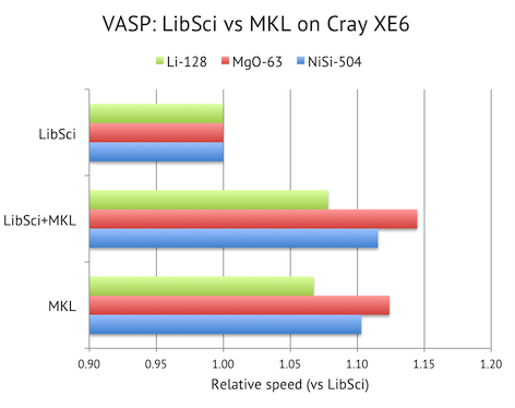
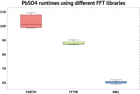
Normally, you combine libsci with the FFTW library. But I would recommend using the FFT routines from MKL instead, since they result in 10-15% faster overall speed in my benchmarks. Recent versions of MKL comes with FFTW3-compatible wrappers built-in (you don’t need to compile them separately), so by linking with MKL and libsci in the correct order, you get the best from both worlds.

VASP 5 lib

Compiling the VASP 5 library is straightforward. It contains some timing and IO routines, necessary for VASP, and LINPACK. My heavy edited makefile looks like this:

.SUFFIXES: .inc .f .F
#-----------------------------------------------------------------------
# Makefile for VASP 5 library on Cray XE6 Lindgren at PDC
#-----------------------------------------------------------------------

# C-preprocessor
CPP     = gcc -E -P -C -DLONGCHAR $*.F >$*.f
FC= ftn

CFLAGS = -O
FFLAGS = -O1 -FI
FREE   =  -FR

DOBJ =  preclib.o timing_.o derrf_.o dclock_.o  diolib.o dlexlib.o drdatab.o


#-----------------------------------------------------------------------
# general rules
#-----------------------------------------------------------------------

libdmy.a: $(DOBJ) linpack_double.o
    -rm libdmy.a
    ar vq libdmy.a $(DOBJ)

linpack_double.o: linpack_double.f
    $(FC) $(FFLAGS) $(NOFREE) -c linpack_double.f

.c.o:
    $(CC) $(CFLAGS) -c $*.c
.F.o:
    $(CPP) 
    $(FC) $(FFLAGS) $(FREE) $(INCS) -c $*.f
.F.f:
    $(CPP) 
.f.o:
    $(FC) $(FFLAGS) $(FREE) $(INCS) -c $*.f

Note that the Fortran compiler is always called “ftn” on the Cray (regardless of the module loaded), and the addition of the “-DLONGCHAR” flag on the CPP line. It activates the longer input format for INCAR files, e.g. you can have MAGMOM lines with more than 256 characters. Now compile the library with the “make” command and check that you have the “libdmy.a” output file. Leave the file here, as the main VASP makefile will include it directly from here.

Editing the main VASP makefile

I suggest that you start from the Linux/Intel Fortran makefile:

cp makefile.linux_ifc_P4 makefile

It is important to realise that the makefile is split in two parts, and is intended to be used in an overriding fashion. If you don’t want to compile the serial version, you should enable the definitions of FC, CPP etc in the second half of the makefile to enable parallel compilation. These will then override the settings for the serial version.

Start by editing the Fortran compiler and its flags:

FC=ftn -I$(MKL_ROOT)/include/fftw 
FFLAGS =  -FR -lowercase -assume byterecl

On Lindgren, I don’t get MKL_ROOT set by default when I load the PrgEnv-intel module, so you might have to do it by yourself too:

MKL_ROOT=/pdc/vol/i-compilers/12.1.5/composer_xe_2011_sp1.11.339/mkl

The step above is site-specific, so you should check where the Intel compilers are actually installed. If you cannot find any documentation, try inspecting the PATH after loading the module.

Then, we change the optimisation flags:

OFLAG=-O2 -ip 

Note that we leave out any SSE/architectural flags, since these are provided automatically by the “xtpe-mc12” module (make sure that it is loaded by checking the output of module list).

We do a similar trick for BLAS/LAPACK by providing empty definitions for them:

# BLAS/LAPACK should be linked automatically by libsci module
BLAS=
LAPACK=

We need to edit the LINK variable to include Intel’s MKL. I also like to add more verbose output of the linking process, to check that I am linking the correct library. One simple way to do this is to ask the linker to say from where it picks up the ZGEMM subroutine (it should be from Cray’s libsci, not MKL).

LINK = -mkl=sequential -Wl,-yzgemm_

Now, move further down in the makefile, to the MPI section, and edit the preprocessors flags:

CPP    = $(CPP_) -DMPI  -DHOST=\"PDC-REGULAR-B01\" -DIFC \
   -DCACHE_SIZE=4000 -DPGF90 -Davoidalloc -DNGZhalf \
   -DMPI_BLOCK=262144 -Duse_collective -DscaLAPACK \
   -DRPROMU_DGEMV  -DRACCMU_DGEMV -DnoSTOPCAR

CACHE_SIZE is only relevant for Furth FFTs, which we do not use. The HOST variable is written out in the top of the OUTCAR file. It can be anything which helps you identify this compilation of VASP. The MPI_BLOCK variable needs to be set higher for best performance on the Cray XE6 interconnect. And finally, “noSTOPCAR” will disable the ability to stop a calculation by using the STOPCAR file. We do this to improve file I/O against the global file systems. (Otherwise, each VASP process will have to check this file for every SCF iteration.)

We will get Cray’s SCALAPACK linked in via libsci, so we set an empty SCA variable:

# SCALAPACK is linked automatically by libsci module
SCA= 

Then activate the parallelized version of the fast Fourier transforms with FFTW bindings:

FFT3D   = fftmpiw.o fftmpi_map.o fftw3d.o fft3dlib.o

Note that we do not need to link to FFTW explicitly, since it is included in MKL.

Finally, we uncomment the last library section for completeness:

LIB     = -L../vasp.5.lib -ldmy  \
      ../vasp.5.lib/linpack_double.o \
      $(SCA) $(LAPACK) $(BLAS)

The full makefile is provided here.

Compiling

VASP does not have a makefile that supports parallel compilation. So in order to compile we just do:

make

If you really want to speed it up, you can try something like:

make -j4; make -j4; make -j4; make -j4;

Run these commands repeatedly until all the compiler errors are cleared (or write a loop in the bash shell). Obviously, this approach only works if you have a makefile that you know works from the start. When finished, you should find a binary called “vasp”.

Running

The Cray compiler environment produces statically linked binaries by default, since this is the most convenient way to run on the Cray compute nodes, so we just have to put e.g. the following in the job script to run on 384 cores (16 compute nodes).

aprun -n 384 /path/to/vasp

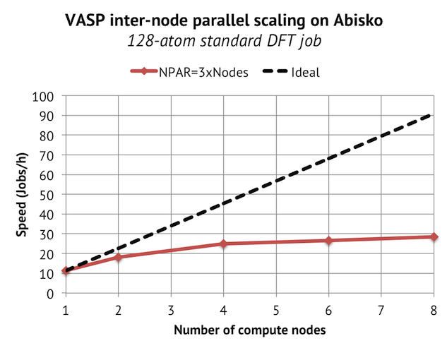
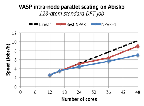
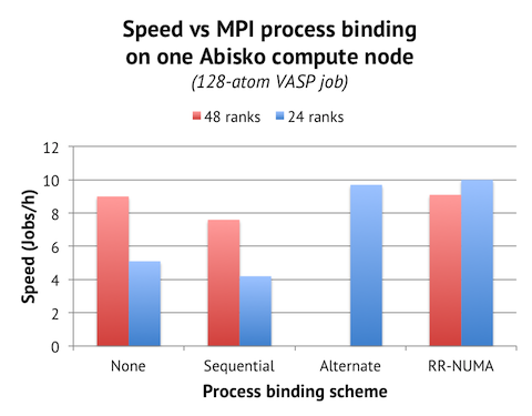
I recommend setting NPAR equal to the number of compute nodes on the Cray XE6. As I have shown before, it is possible to run really big VASP simulations on the Cray with decent scaling over 1000-2000 cores. If you go beyond 32 compute nodes, it is worth trying to run on only half the number of cores per node. So on a machine with 24 cores per node, you would ask for 768 cores, but actually run like this:

aprun -n 384 -N 12 -S 3 /path/to/vasp

Tuning VASP: Fast Fourier Transforms

This is the first post in a series about VASP tuning. Optimized Fast Fourier transform subroutines are one of the keystones of getting a fast VASP installation. When I did a similar study for the Matter cluster at NSC (which has Intel “Nehalem” processors) in 2011, I found that MKL was superior. Now, it is time to look at Triolith, which has processors of “Sandy Bridge” architecture. These processors have new 256-bit vector instructions (called “AVX”), which need to be exploited for maximum floating-point performance.

Basically, we have three choices of FFTs:

  • VASP’s built-in library by Jürgen Furthmüller, called “FURTH”. It is quite old now, but has the advantage that it comes with the VASP code, so that we don’t have to rely on an external library; we can also recompile it for new architectures. For best performance, one have to optimize the CACHE_SIZE precompiler flag (usually a value between 0-32000).
  • The classical FFTW library. It can be optimized for many architectures by an automatic procedure. FFTW has support for AVX since version 3.3.1. On Triolith, we currently have version 3.3.2.
  • Intel’s own Math Kernel Library (“MKL”). Presumably, noone should be better at optimizing for Intel processors than Intel themselves? Intel is also very aggressive with processor support, and many times MKL has support for unreleased processors. MKL gained AVX support in version 10.2, but version 10.3 and higher uses AVX instructions automatically.

I chose the PbSO4 cell with 24 atoms as the test system, as it is quite small and more reliant on good FFT performance. Here are the results, without much further ado:

Runtimes of VASP with different FFT libraries

We can see that MKL 10.3 is the best choice here, with an average runtime of 61 seconds, 45% faster than FFTW 3.3.2. The results for FFT-FURTH does not come out well. I think one reason is that this library does not utilize AVX instructions fully on Sandy Bridge. The default optimization options in the makefile are very conservative (-O1/-O2), so we will not get the full benefit. It might be possible to compile it more aggressively and get better speed.