

There are just a few implementations of the PAW method: PWPAW, ABINIT, VASP, GPAW, and in the PWscf program in Quantum Espresso (“QE” from now on). VASP is frequently held up as the fastest implementation, and I concluded in earlier tests that standard DFT in ABINIT is too slow compared to VASP to be useful for when running large supercells. But how does QE compare to VASP? There has been extensive work on QE in the last years, such as adding GPU support and mixed OpenMP/MPI parallelism, and you can find papers showing good parallel scalability such as (ref1) and (ref2). By request, I will therefore perform and publish some comparisons of VASP and QE, in the context of PAW calculations. Primarily, I am interesting in:
- Raw speed, measured as performance on a single 16 core compute node.
- Parallel scalability, measured as the time to solution and computational efficiency for very large supercell calculations.
- General robustness and production readiness, in particular numerical stability, sane defaults, and quality of documentation.
So as the first step, before going into parallel scaling studies, it is useful to know the performance on the level of a single compute node. In the ABINIT vs VASP study, I used a silicon supercell with 31 atoms and one vacancy for basic testing. I will use it here as well to provide a point of reference.
Methods
Access to prepared PAW dataset is crucial for a PAW code to be useful, as most users prefer to not generate pseudopotentials themselves (although it can be discussed whether this is a wise approach). Fortunately, there are now more PAW datasets available for QE. I found “Si.pbe-n-kjpaw_psl.0.1.UPF” to be the most similar one to VASP’s standard silicon POTCAR. It is a scalar relativistic setup with 4 valance electrons for the PBE exchange-correlation functional. It differs in the suggested plane-wave cutoff, though, where the QE value is much higher (13.8 Ry, ca 500 eV) compared to the VASP one (250 eV). I decided to use 250 eV in both programs for benchmarking purposes, but it is a highly relevant question if you get the same physical results at this cutoff? I will postpone the discussion of differences between PAW potentials for now, but I expect to return to it at a later time.
As usual, I put some effort into making sure that I am running as similar calculations as possible from a numerical point of view:
- The plane-wave cutoff was set to 18.4 Ry/250 eV. This lead to a 72x72x72 coarse FFT grid in both programs.
- The fine FFT grids were 144x144x144.
- 80 bands, set manually
- 6 k-points (automatically generated)
- 6 symmetry operations detected in the crystal lattice
- SCF convergence thresholds were 1.0e-6 Ry and 1.0e-5 eV, respectively.
- Minimal disk I/O (i.e. no writing of WAVECAR and wfc files).
A notable difference is that PWscf does not have the RMM-DIIS algorithm, instead I used the default Davidson iterative diagonalization. In the VASP calculations, I used the hybrid Davidson/RMM-DIIS approach (ALGO=fast), which is what I would use in a real-life scenario.
VASP was compiled with the -DNGZhalf preprocessor option for improved FFT performance. I could not find a clear answer in the PWscf documentation about this feature, but it does use the real FFT representation for gamma point calculations, so I presume that the “half” representation is also employed for normal calculations.
Results
Results when running the Si 31 atom cell on 1 Triolith compute node (16 Xeon E5 cores clocked at 2.2-3.0 Ghz):
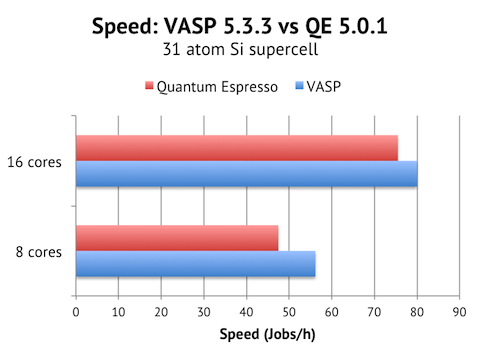
It is great to find VASP and QE pretty much tied for this test case. VASP is around 6% faster, but the QE calculation also required 20 SCF steps instead of 15 steps in VASP, so it is possible that a more experienced QE user would be able to tune the SCF convergence better to achieve at least parity in speed.
I ran with both 8 cores and 16 cores per node to get a feel for the intra-node parallel scaling. QE actually scales better with 1.6x speed-up from 8 to 16 cores, vs 1.3x for VASP. This indicates to me that QE puts less pressure on the memory system and could scale better on big multicore nodes.
I also tested the OpenMP enabled version of QE, but for this test case there was no real benefit in terms of speed: 8 MPI ranks with 2 OpenMP threads each did run faster (+27%) than 8 ranks with only MPI, but not as fast as with 16 MPI ranks. But there was a slight reduction in memory: 16 MPI ranks with -npool 2 required a maximum of 678 MB of memory, whereas 8 MPI ranks with 2 OpenMP threads used only 605 MB. So by using this approach, you could save some memory at the expense of speed. VASP, for comparison, used 1205 MB with k-point parallelization with 16 ranks, but 706 MB with band parallelization (which was the fastest option), so the memory usage of QE and VASP is very similar in practice.
Summary
In conclusion, this was my first serious calculations with PWscf and my overall impression is that the PAW speed is promising, and that it was relatively painless to set up the calculation and get going. I found the documentation comprehensive, but somewhat lacking in organization and mostly of reference kind. There are no explicit examples or practical notes of what you actually need to do to run a typical calculation. In fact, in my first attempt, I completely failed at getting PWscf to read my input files — I had to consult with an experienced QE user to understand why QE would not read my atomic positions (it turned out that the ATOMIC_POSITIONS section is only read if “nat” is set in the SYSTEM section). Once over the initial hurdle, it was a quite smooth ride, though. SCF convergence was achieved using the default settings, and all symmetries were detected correctly: that is something you cannot take for granted in all electronic structure codes.
Next up is a medium-sized calculation, the Li2FeSiO4 supercell with 128 atoms.